Chapter 4 Selection scheme diagnostic experiments

experiment_slug <- "2023-05-10-diagnostics"

working_directory <- paste0(
  "experiments/",
  experiment_slug,
  "/analysis/"
)

if (exists("bookdown_wd_prefix")) {
  working_directory <- paste0(
    bookdown_wd_prefix,
    working_directory
  )
}

4.1 Dependencies

library(tidyverse)

## ── Attaching packages ──────────────────────────────────────────────────────────────────────────────────────────────────────────────────────────────────────────────────────────────────────────────────────── tidyverse 1.3.2 ──
## ✔ ggplot2 3.3.6     ✔ purrr   1.0.1
## ✔ tibble  3.1.8     ✔ dplyr   1.1.0
## ✔ tidyr   1.3.0     ✔ stringr 1.5.0
## ✔ readr   2.1.3     ✔ forcats 0.5.2
## ── Conflicts ─────────────────────────────────────────────────────────────────────────────────────────────────────────────────────────────────────────────────────────────────────────────────────────── tidyverse_conflicts() ──
## ✖ dplyr::filter() masks stats::filter()
## ✖ dplyr::lag()    masks stats::lag()

library(ggplot2)
library(cowplot)
library(RColorBrewer)
library(khroma)
library(rstatix)

## 
## Attaching package: 'rstatix'
## 
## The following object is masked from 'package:stats':
## 
##     filter

library(knitr)
source("https://gist.githubusercontent.com/benmarwick/2a1bb0133ff568cbe28d/raw/fb53bd97121f7f9ce947837ef1a4c65a73bffb3f/geom_flat_violin.R")

print(version)

##                _                           
## platform       aarch64-apple-darwin20      
## arch           aarch64                     
## os             darwin20                    
## system         aarch64, darwin20           
## status                                     
## major          4                           
## minor          2.1                         
## year           2022                        
## month          06                          
## day            23                          
## svn rev        82513                       
## language       R                           
## version.string R version 4.2.1 (2022-06-23)
## nickname       Funny-Looking Kid

4.2 Setup

# Configure our default graphing theme
theme_set(theme_cowplot())
# Create a directory to store plots
plot_directory <- paste0(working_directory, "plots/")
dir.create(plot_directory, showWarnings=FALSE)

4.2.1 Load experiment summary data

summary_data_loc <- paste0(working_directory, "data/aggregate.csv")
summary_data <- read_csv(summary_data_loc)

## Rows: 520 Columns: 49
## ── Column specification ─────────────────────────────────────────────────────────────────────────────────────────────────────────────────────────────────────────────────────────────────────────────────────────────────────────
## Delimiter: ","
## chr  (5): DIAGNOSTIC, EVAL_FIT_EST_MODE, EVAL_MODE, SELECTION, STOP_MODE
## dbl (44): ACCURACY, CREDIT, DIAGNOSTIC_DIMENSIONALITY, GENE_LOWER_BND, GENE_...
## 
## ℹ Use `spec()` to retrieve the full column specification for this data.
## ℹ Specify the column types or set `show_col_types = FALSE` to quiet this message.

summary_data <- summary_data %>%
  mutate(
    eval_mode_row = case_when(
      EVAL_MODE == "full" & TEST_DOWNSAMPLE_RATE == "1" ~ "down-sample",
      EVAL_MODE == "full" & NUM_COHORTS == "1" ~ "cohort",
      .default = EVAL_MODE
    ),
    evals_per_gen = case_when(
      EVAL_MODE == "cohort-full-compete" ~ 1.0 / NUM_COHORTS,
      EVAL_MODE == "cohort" ~ 1.0 / NUM_COHORTS,
      EVAL_MODE == "down-sample" ~ TEST_DOWNSAMPLE_RATE,
      EVAL_MODE == "full" ~ 1.0
    ),
    EVAL_FIT_EST_MODE = case_when(
      EVAL_FIT_EST_MODE == "ancestor-opt" ~ "ancestor",
      EVAL_FIT_EST_MODE == "relative-opt" ~ "relative",
      .default = EVAL_FIT_EST_MODE
    ),
    .keep = "all"
  ) %>%
  mutate(
    evals_per_gen = as.factor(evals_per_gen),
    eval_mode_row = as.factor(eval_mode_row),
    DIAGNOSTIC = as.factor(DIAGNOSTIC),
    SELECTION = as.factor(SELECTION),
    EVAL_MODE = as.factor(EVAL_MODE),
    NUM_COHORTS = as.factor(NUM_COHORTS),
    TEST_DOWNSAMPLE_RATE = as.factor(TEST_DOWNSAMPLE_RATE),
    EVAL_FIT_EST_MODE = factor(
      EVAL_FIT_EST_MODE,
      levels = c(
        "none",
        "ancestor",
        "relative"
      ),
      labels = c(
        "None",
        "Ancestor",
        "Relative"
      )
    )
  )

# Split summary data on diagnostic
con_obj_summary_data <- filter(
  summary_data,
  DIAGNOSTIC == "contradictory-objectives"
)

explore_summary_data <- filter(
  summary_data,
  DIAGNOSTIC == "multipath-exploration"
)

4.2.2 Load experiment time series data

ts_data_loc <- paste0(working_directory, "data/time_series.csv")
ts_data <- read_csv(ts_data_loc)

## Rows: 104000 Columns: 19
## ── Column specification ─────────────────────────────────────────────────────────────────────────────────────────────────────────────────────────────────────────────────────────────────────────────────────────────────────────
## Delimiter: ","
## chr  (4): DIAGNOSTIC, EVAL_FIT_EST_MODE, EVAL_MODE, SELECTION
## dbl (15): NUM_COHORTS, SEED, TEST_DOWNSAMPLE_RATE, entropy_selected_ids, eva...
## 
## ℹ Use `spec()` to retrieve the full column specification for this data.
## ℹ Specify the column types or set `show_col_types = FALSE` to quiet this message.

ts_data <- ts_data %>%
  mutate(
    eval_mode_row = case_when(
      EVAL_MODE == "full" & TEST_DOWNSAMPLE_RATE == "1" ~ "down-sample",
      EVAL_MODE == "full" & NUM_COHORTS == "1" ~ "cohort",
      .default = EVAL_MODE
    ),
    evals_per_gen = case_when(
      EVAL_MODE == "cohort-full-compete" ~ 1.0 / NUM_COHORTS,
      EVAL_MODE == "cohort" ~ 1.0 / NUM_COHORTS,
      EVAL_MODE == "down-sample" ~ TEST_DOWNSAMPLE_RATE,
      EVAL_MODE == "full" ~ 1.0
    ),
    EVAL_FIT_EST_MODE = case_when(
      EVAL_FIT_EST_MODE == "ancestor-opt" ~ "ancestor",
      EVAL_FIT_EST_MODE == "relative-opt" ~ "relative",
      .default = EVAL_FIT_EST_MODE
    ),
    .keep = "all"
  ) %>%
  mutate(
    evals_per_gen = as.factor(evals_per_gen),
    DIAGNOSTIC = as.factor(DIAGNOSTIC),
    SELECTION = as.factor(SELECTION),
    EVAL_MODE = as.factor(EVAL_MODE),
    NUM_COHORTS = as.factor(NUM_COHORTS),
    TEST_DOWNSAMPLE_RATE = as.factor(TEST_DOWNSAMPLE_RATE),
    EVAL_FIT_EST_MODE = factor(
      EVAL_FIT_EST_MODE,
      levels = c(
        "none",
        "ancestor",
        "relative"
      ),
      labels = c(
        "None",
        "Ancestor",
        "Relative"
      )
    )
  )

con_obj_ts_data <- ts_data %>%
  filter(DIAGNOSTIC == "contradictory-objectives")

explore_ts_data <- ts_data %>%
  filter(DIAGNOSTIC == "multipath-exploration")

4.2.3 Load estimate source distributions

est_source_data <- read_csv(
  paste0(working_directory, "data/phylo-est-info.csv")
)

## Rows: 520 Columns: 38
## ── Column specification ─────────────────────────────────────────────────────────────────────────────────────────────────────────────────────────────────────────────────────────────────────────────────────────────────────────
## Delimiter: ","
## chr  (6): OUTPUT_DIR, DIAGNOSTIC, STOP_MODE, SELECTION, EVAL_MODE, EVAL_FIT_...
## dbl (32): SNAPSHOT_INTERVAL, OUTPUT_SUMMARY_DATA_INTERVAL, MUTATE_STD, TARGE...
## 
## ℹ Use `spec()` to retrieve the full column specification for this data.
## ℹ Specify the column types or set `show_col_types = FALSE` to quiet this message.

est_source_data <- est_source_data %>%
  mutate(
    eval_mode_row = case_when(
      EVAL_MODE == "full" & TEST_DOWNSAMPLE_RATE == "1" ~ "down-sample",
      EVAL_MODE == "full" & NUM_COHORTS == "1" ~ "cohort",
      .default = EVAL_MODE
    ),
    evals_per_gen = case_when(
      EVAL_MODE == "cohort-full-compete" ~ 1.0 / NUM_COHORTS,
      EVAL_MODE == "cohort" ~ 1.0 / NUM_COHORTS,
      EVAL_MODE == "down-sample" ~ TEST_DOWNSAMPLE_RATE,
      EVAL_MODE == "full" ~ 1.0
    ),
    EVAL_FIT_EST_MODE = case_when(
      EVAL_FIT_EST_MODE == "ancestor-opt" ~ "ancestor",
      EVAL_FIT_EST_MODE == "relative-opt" ~ "relative",
      .default = EVAL_FIT_EST_MODE
    ),
    .keep = "all"
  ) %>%
  mutate(
    evals_per_gen = as.factor(evals_per_gen),
    eval_mode_row = as.factor(eval_mode_row),
    DIAGNOSTIC = as.factor(DIAGNOSTIC),
    SELECTION = as.factor(SELECTION),
    EVAL_MODE = as.factor(EVAL_MODE),
    NUM_COHORTS = as.factor(NUM_COHORTS),
    TEST_DOWNSAMPLE_RATE = as.factor(TEST_DOWNSAMPLE_RATE),
    EVAL_FIT_EST_MODE = factor(
      EVAL_FIT_EST_MODE,
      levels = c(
        "none",
        "ancestor",
        "relative"
      ),
      labels = c(
        "None",
        "Ancestor",
        "Relative"
      )
    )
  ) %>%
  mutate(
    prop_self_lookups = case_when(
      (EVAL_MODE != "full" & EVAL_FIT_EST_MODE != "None") ~
        self_count / (other_count + ancestor_count + descendant_count + self_count + outside_count),
      .default = 0
    ),
    prop_other_lookups =  case_when(
      (EVAL_MODE != "full" & EVAL_FIT_EST_MODE != "None") ~
        other_count / (other_count + ancestor_count + descendant_count + self_count + outside_count),
      .default = 0
    ),
    prop_ancestor_lookups =  case_when(
      (EVAL_MODE != "full" & EVAL_FIT_EST_MODE != "None") ~
        ancestor_count / (other_count + ancestor_count + descendant_count + self_count + outside_count),
      .default = 0
    ),
    prop_descendant_lookups = case_when(
      (EVAL_MODE != "full" & EVAL_FIT_EST_MODE != "None") ~
        descendant_count / (other_count + ancestor_count + descendant_count + self_count + outside_count),
      .default = 0
    ),
    prop_outside_lookups =  case_when(
      (EVAL_MODE != "full" & EVAL_FIT_EST_MODE != "None") ~
        outside_count / (other_count + ancestor_count + descendant_count + self_count + outside_count),
      .default = 0
    )
  )

4.3 Contradictory objectives diagnostic

4.3.1 Population-wide satisfactory trait coverage (final)

Satifactory trait coverage after 50,000 generations:

contradictory_obj_final_plt <- ggplot(
    con_obj_summary_data,
    aes(
      x = EVAL_FIT_EST_MODE,
      y = pop_optimal_trait_coverage,
      fill = EVAL_FIT_EST_MODE
    )
  ) +
  geom_flat_violin(
    position = position_nudge(x = .2, y = 0),
    alpha = .8,
    adjust=1.5
  ) +
  geom_point(
    mapping=aes(color=EVAL_FIT_EST_MODE),
    position = position_jitter(width = .15),
    size = .5,
    alpha = 0.8
  ) +
  geom_boxplot(
    width = .1,
    outlier.shape = NA,
    alpha = 0.5
  ) +
  scale_y_continuous(
    # limits = c(-0.5, 100)
  ) +
  scale_fill_bright() +
  scale_color_bright() +
  facet_grid(
    eval_mode_row~evals_per_gen,
    # nrow=2,
    labeller=label_both
  ) +
  theme(
    legend.position = "none",
    axis.text.x = element_text(
      angle = 30,
      hjust = 1
    ),
    panel.border = element_rect(color="gray", size=2)
  )
ggsave(
  filename = paste0(plot_directory, "contra-obj-final.pdf"),
  plot = contradictory_obj_final_plt + labs(title="Contradictory objectives"),
  width = 15,
  height = 10
)

contradictory_obj_final_plt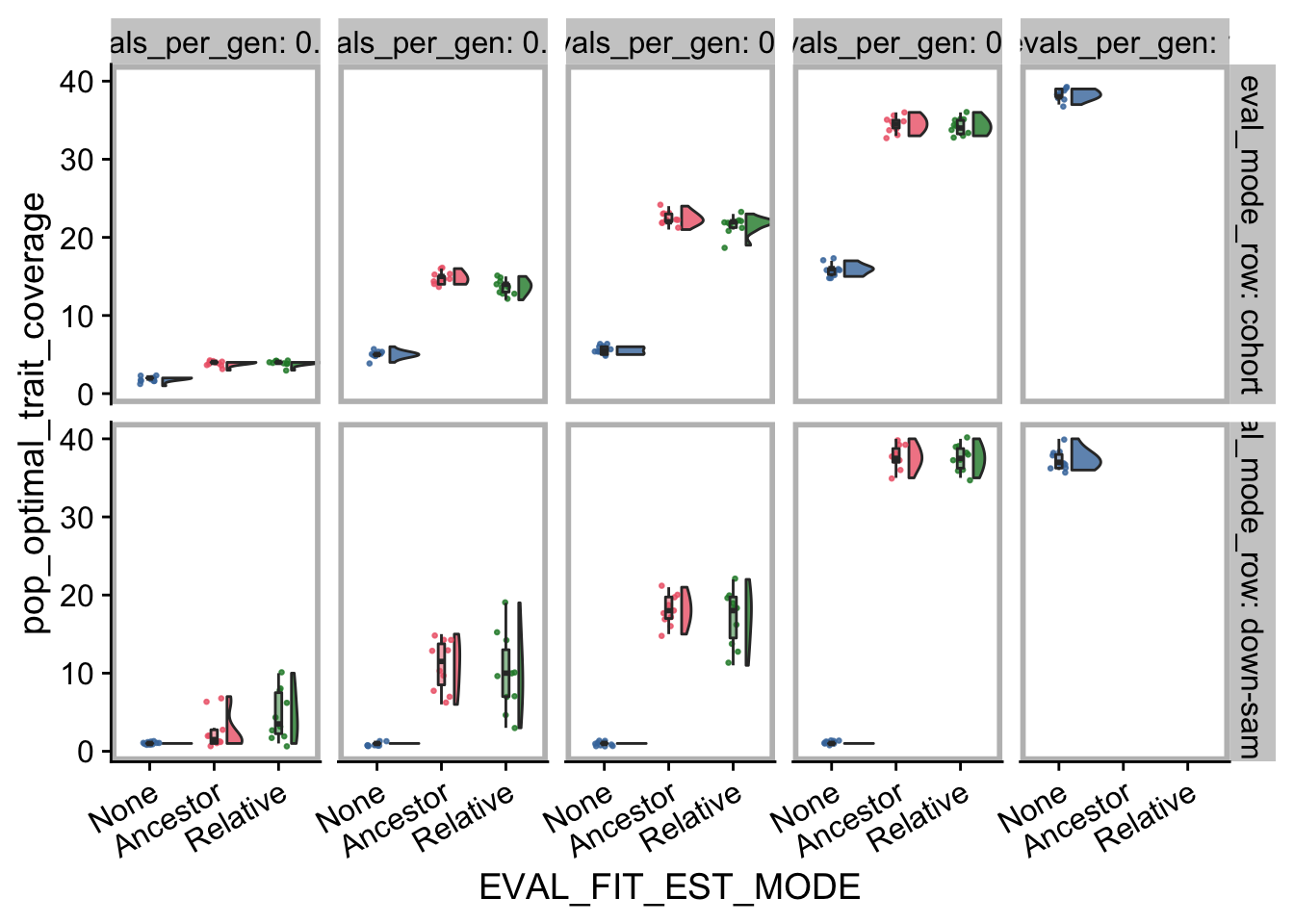

4.3.1.1 Statistical analysis

First, we create a table of summary values for satisfactory trait coverage in the final generation.

con_obj_summary_data %>%
  filter(EVAL_MODE != "full") %>%
  group_by(EVAL_MODE, evals_per_gen, EVAL_FIT_EST_MODE) %>%
  summarize(
    cov_median = median(pop_optimal_trait_coverage),
    cov_mean = mean(pop_optimal_trait_coverage),
    n = n()
  ) %>%
  kable()

## `summarise()` has grouped output by 'EVAL_MODE', 'evals_per_gen'. You can
## override using the `.groups` argument.

EVAL_MODE	evals_per_gen	EVAL_FIT_EST_MODE	cov_median	cov_mean	n
cohort	0.01	None	2.0	1.9	10
cohort	0.01	Ancestor	4.0	3.9	10
cohort	0.01	Relative	4.0	3.9	10
cohort	0.05	None	5.0	5.0	10
cohort	0.05	Ancestor	15.0	14.8	10
cohort	0.05	Relative	14.0	13.7	10
cohort	0.1	None	5.5	5.5	10
cohort	0.1	Ancestor	22.0	22.4	10
cohort	0.1	Relative	22.0	21.6	10
cohort	0.5	None	16.0	15.9	10
cohort	0.5	Ancestor	34.5	34.5	10
cohort	0.5	Relative	34.0	34.2	10
down-sample	0.01	None	1.0	1.0	10
down-sample	0.01	Ancestor	1.5	2.5	10
down-sample	0.01	Relative	3.5	4.7	10
down-sample	0.05	None	1.0	1.0	10
down-sample	0.05	Ancestor	11.5	11.0	10
down-sample	0.05	Relative	10.0	10.0	10
down-sample	0.1	None	1.0	1.0	10
down-sample	0.1	Ancestor	18.0	18.1	10
down-sample	0.1	Relative	18.0	17.1	10
down-sample	0.5	None	1.0	1.0	10
down-sample	0.5	Ancestor	37.5	37.6	10
down-sample	0.5	Relative	37.5	37.5	10

Next, we perform a Kruskal-Wallis test to determine which comparisons contain statistically significant differences among treatments.

con_obj_kw_test <- con_obj_summary_data %>%
  filter(EVAL_MODE != "full") %>%
  group_by(EVAL_MODE, evals_per_gen) %>%
  kruskal_test(pop_optimal_trait_coverage ~ EVAL_FIT_EST_MODE) %>%
  unite(
    "comparison_group",
    EVAL_MODE,
    evals_per_gen,
    sep = "_",
    remove = FALSE
  )

kable(con_obj_kw_test)

comparison_group	EVAL_MODE	evals_per_gen	.y.	n	statistic	df	p	method
cohort_0.01	cohort	0.01	pop_optimal_trait_coverage	30	25.55066	2	2.80e-06	Kruskal-Wallis
cohort_0.05	cohort	0.05	pop_optimal_trait_coverage	30	22.72918	2	1.16e-05	Kruskal-Wallis
cohort_0.1	cohort	0.1	pop_optimal_trait_coverage	30	21.76615	2	1.88e-05	Kruskal-Wallis
cohort_0.5	cohort	0.5	pop_optimal_trait_coverage	30	20.05082	2	4.43e-05	Kruskal-Wallis
down-sample_0.01	down-sample	0.01	pop_optimal_trait_coverage	30	15.17863	2	5.06e-04	Kruskal-Wallis
down-sample_0.05	down-sample	0.05	pop_optimal_trait_coverage	30	20.38430	2	3.75e-05	Kruskal-Wallis
down-sample_0.1	down-sample	0.1	pop_optimal_trait_coverage	30	20.29663	2	3.91e-05	Kruskal-Wallis
down-sample_0.5	down-sample	0.5	pop_optimal_trait_coverage	30	20.31895	2	3.87e-05	Kruskal-Wallis

Finally, we perform a pairwise Wilcoxon rank-sum test (using a Holm-Bonferroni correction for multiple comparisons). Note that only results from signific

sig_kw_groups <- filter(con_obj_kw_test, p < 0.05)$comparison_group

con_obj_stats <- con_obj_summary_data %>%
  unite(
    "comparison_group",
    EVAL_MODE,
    evals_per_gen,
    sep = "_",
    remove = FALSE
  ) %>%
  filter(EVAL_MODE != "full" & comparison_group %in% sig_kw_groups) %>%
  group_by(EVAL_MODE, evals_per_gen) %>%
  pairwise_wilcox_test(pop_optimal_trait_coverage ~ EVAL_FIT_EST_MODE) %>%
  adjust_pvalue(method = "holm") %>%
  add_significance("p.adj")

kable(con_obj_stats)

EVAL_MODE	evals_per_gen	.y.	group1	group2	n1	n2	statistic	p	p.adj	p.adj.signif
cohort	0.01	pop_optimal_trait_coverage	None	Ancestor	10	10	0.0	3.58e-05	0.0008592	***
cohort	0.01	pop_optimal_trait_coverage	None	Relative	10	10	0.0	3.58e-05	0.0008592	***
cohort	0.01	pop_optimal_trait_coverage	Ancestor	Relative	10	10	50.0	1.00e+00	1.0000000	ns
cohort	0.05	pop_optimal_trait_coverage	None	Ancestor	10	10	0.0	9.66e-05	0.0015456	**
cohort	0.05	pop_optimal_trait_coverage	None	Relative	10	10	0.0	1.00e-04	0.0015456	**
cohort	0.05	pop_optimal_trait_coverage	Ancestor	Relative	10	10	80.0	1.90e-02	0.1520000	ns
cohort	0.1	pop_optimal_trait_coverage	None	Ancestor	10	10	0.0	1.25e-04	0.0016250	**
cohort	0.1	pop_optimal_trait_coverage	None	Relative	10	10	0.0	1.16e-04	0.0016240	**
cohort	0.1	pop_optimal_trait_coverage	Ancestor	Relative	10	10	70.5	9.60e-02	0.5760000	ns
cohort	0.5	pop_optimal_trait_coverage	None	Ancestor	10	10	0.0	1.49e-04	0.0017760	**
cohort	0.5	pop_optimal_trait_coverage	None	Relative	10	10	0.0	1.48e-04	0.0017760	**
cohort	0.5	pop_optimal_trait_coverage	Ancestor	Relative	10	10	58.0	5.56e-01	1.0000000	ns
down-sample	0.01	pop_optimal_trait_coverage	None	Ancestor	10	10	25.0	1.50e-02	0.1350000	ns
down-sample	0.01	pop_optimal_trait_coverage	None	Relative	10	10	5.0	2.27e-04	0.0022700	**
down-sample	0.01	pop_optimal_trait_coverage	Ancestor	Relative	10	10	24.0	4.90e-02	0.3430000	ns
down-sample	0.05	pop_optimal_trait_coverage	None	Ancestor	10	10	0.0	6.25e-05	0.0013442	**
down-sample	0.05	pop_optimal_trait_coverage	None	Relative	10	10	0.0	6.16e-05	0.0013442	**
down-sample	0.05	pop_optimal_trait_coverage	Ancestor	Relative	10	10	57.5	5.92e-01	1.0000000	ns
down-sample	0.1	pop_optimal_trait_coverage	None	Ancestor	10	10	0.0	6.25e-05	0.0013442	**
down-sample	0.1	pop_optimal_trait_coverage	None	Relative	10	10	0.0	6.29e-05	0.0013442	**
down-sample	0.1	pop_optimal_trait_coverage	Ancestor	Relative	10	10	56.0	6.75e-01	1.0000000	ns
down-sample	0.5	pop_optimal_trait_coverage	None	Ancestor	10	10	0.0	6.11e-05	0.0013442	**
down-sample	0.5	pop_optimal_trait_coverage	None	Relative	10	10	0.0	6.20e-05	0.0013442	**
down-sample	0.5	pop_optimal_trait_coverage	Ancestor	Relative	10	10	52.0	9.08e-01	1.0000000	ns

# con_obj_stats %>%
#   filter(p.adj <= 0.05) %>%
#   arrange(
#     desc(p.adj)
#   ) %>%
#   kable()

4.3.2 Population-wide satisfactory trait coverage (over time)

contradictory_obj_pop_cov_ts <- ggplot(
    con_obj_ts_data,
    aes(
      x = ts_step,
      y = pop_optimal_trait_coverage,
      fill = EVAL_FIT_EST_MODE,
      color = EVAL_FIT_EST_MODE
    )
  ) +
  stat_summary(
    geom = "line",
    fun = mean
  ) +
  stat_summary(
    geom = "ribbon",
    fun.data = "mean_cl_boot",
    fun.args = list(conf.int = 0.95),
    alpha = 0.2,
    linetype = 0
  ) +
  scale_fill_bright() +
  scale_color_bright() +
  facet_wrap(
    EVAL_MODE ~ evals_per_gen,
    ncol = 1,
    labeller = label_both
  ) +
  theme(
    legend.position = "bottom"
  )

ggsave(
  filename = paste0(plot_directory, "contra-obj-ts.pdf"),
  plot = contradictory_obj_pop_cov_ts + labs(title="Contradictory objectives"),
  width = 10,
  height = 15
)

contradictory_obj_pop_cov_ts

4.3.3 Phylogeny estimate source distributions

est_source_data %>%
  filter(DIAGNOSTIC == "contradictory-objectives") %>%
  filter(EVAL_MODE != "full" & EVAL_FIT_EST_MODE != "None") %>%
  ggplot(
      aes(
        x = EVAL_FIT_EST_MODE,
        y = prop_self_lookups
      )
    ) +
    geom_boxplot() +
    geom_point() +
    facet_grid(
      cols = vars(evals_per_gen),
      rows = vars(EVAL_MODE),
      labeller = label_both
    ) +
    scale_y_continuous("Proportion of self lookups") +
    scale_x_discrete("Evaluations per generation") +
    theme_bw() +
    theme(legend.position = "none")

ggsave(
   filename=paste0(plot_directory, "contra-obj-self-lookups.pdf")
)

## Saving 7 x 5 in image

est_source_data %>%
  filter(DIAGNOSTIC == "contradictory-objectives") %>%
  filter(EVAL_MODE != "full" & EVAL_FIT_EST_MODE != "None") %>%
  ggplot(
      aes(
        x = EVAL_FIT_EST_MODE,
        y = prop_ancestor_lookups
      )
    ) +
    geom_boxplot() +
    geom_point() +
    facet_grid(
      cols = vars(evals_per_gen),
      rows = vars(EVAL_MODE),
      labeller = label_both
    ) +
    scale_y_continuous("Proportion of ancestor lookups") +
    scale_x_discrete("Evaluations per generation") +
    theme_bw() +
    theme(legend.position = "none")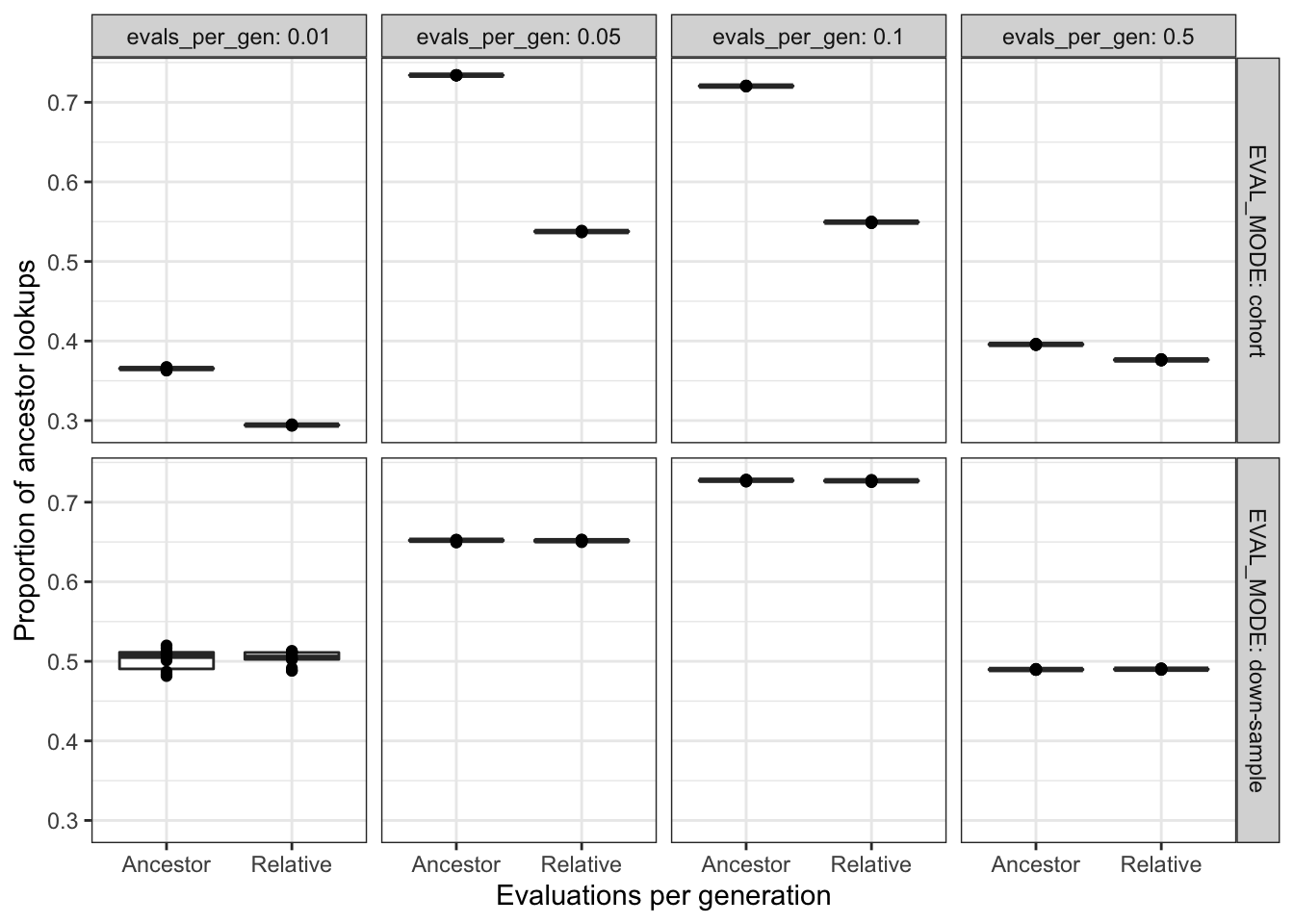

ggsave(
   filename=paste0(plot_directory, "contra-obj-ancestor-lookups.pdf")
)

## Saving 7 x 5 in image

est_source_data %>%
  filter(DIAGNOSTIC == "contradictory-objectives") %>%
  filter(EVAL_MODE != "full" & EVAL_FIT_EST_MODE != "None") %>%
  ggplot(
      aes(
        x = EVAL_FIT_EST_MODE,
        y = prop_descendant_lookups
      )
    ) +
    geom_boxplot() +
    geom_point() +
    facet_grid(
      cols = vars(evals_per_gen),
      rows = vars(EVAL_MODE),
      labeller = label_both
    ) +
    scale_y_continuous("Proportion of descendant lookups") +
    scale_x_discrete("Evaluations per generation") +
    theme_bw() +
    theme(legend.position = "none")

ggsave(
   filename=paste0(plot_directory, "contra-obj-descendant-lookups.pdf")
)

## Saving 7 x 5 in image

est_source_data %>%
  filter(DIAGNOSTIC == "contradictory-objectives") %>%
  filter(EVAL_MODE != "full" & EVAL_FIT_EST_MODE != "None") %>%
  ggplot(
      aes(
        x = EVAL_FIT_EST_MODE,
        y = prop_other_lookups
      )
    ) +
    geom_boxplot() +
    geom_point() +
    facet_grid(
      cols = vars(evals_per_gen),
      rows = vars(EVAL_MODE),
      labeller = label_both
    ) +
    scale_y_continuous("Proportion of other lookups") +
    scale_x_discrete("Evaluations per generation") +
    theme_bw() +
    theme(legend.position = "none")

ggsave(
   filename=paste0(plot_directory, "contra-obj-other-lookups.pdf")
)

## Saving 7 x 5 in image

est_source_data %>%
  filter(DIAGNOSTIC == "contradictory-objectives") %>%
  filter(EVAL_MODE != "full" & EVAL_FIT_EST_MODE != "None") %>%
  ggplot(
      aes(
        x = EVAL_FIT_EST_MODE,
        y = prop_outside_lookups
      )
    ) +
    geom_boxplot() +
    geom_point() +
    facet_grid(
      cols = vars(evals_per_gen),
      rows = vars(EVAL_MODE),
      labeller = label_both
    ) +
    scale_y_continuous("Proportion of outside lookups") +
    scale_x_discrete("Evaluations per generation") +
    theme_bw() +
    theme(legend.position = "none")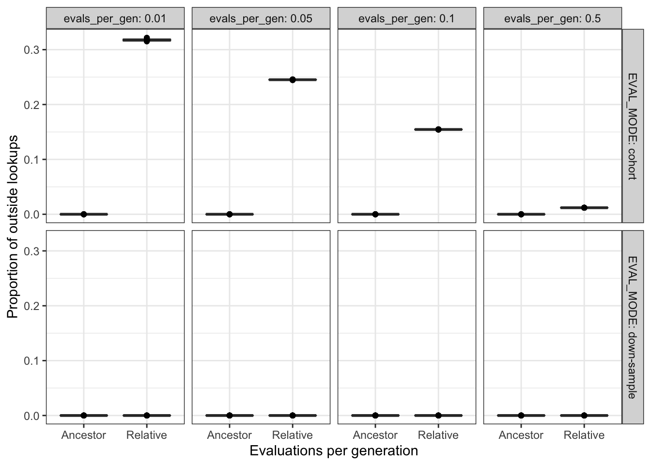

ggsave(
   filename=paste0(plot_directory, "contra-obj-outside-lookups.pdf")
)

## Saving 7 x 5 in image

4.4 Multi-path exploration diagnostic

4.4.1 Maximum aggregate score (final)

explore_final_score_plt <- ggplot(
    explore_summary_data,
    aes(
      x = EVAL_FIT_EST_MODE,
      y = max_agg_score,
      fill = EVAL_FIT_EST_MODE
    )
  ) +
  geom_flat_violin(
    position = position_nudge(x = .2, y = 0),
    alpha = .8,
    adjust=1.5
  ) +
  geom_point(
    mapping=aes(color=EVAL_FIT_EST_MODE),
    position = position_jitter(width = .15),
    size = .5,
    alpha = 0.8
  ) +
  geom_boxplot(
    width = .1,
    outlier.shape = NA,
    alpha = 0.5
  ) +
  scale_y_continuous(
    # limits = c(-0.5, 100)
  ) +
  scale_fill_bright() +
  scale_color_bright() +
  facet_grid(
    eval_mode_row~evals_per_gen,
    # nrow=2,
    labeller=label_both
  ) +
  theme(
    legend.position = "none",
    axis.text.x = element_text(
      angle = 30,
      hjust = 1
    ),
    panel.border = element_rect(color="gray", size=2)
  )
ggsave(
  filename = paste0(plot_directory, "explore-final.pdf"),
  plot = explore_final_score_plt + labs(title="Multi-path exploration"),
  width = 15,
  height = 10
)

4.4.1.1 Statistical analysis

explore_summary_data %>%
  filter(EVAL_MODE != "full") %>%
  group_by(EVAL_MODE, evals_per_gen, EVAL_FIT_EST_MODE) %>%
  summarize(
    score_median = median(max_agg_score),
    score_mean = mean(max_agg_score),
    n = n()
  ) %>%
  kable()

## `summarise()` has grouped output by 'EVAL_MODE', 'evals_per_gen'. You can
## override using the `.groups` argument.

EVAL_MODE	evals_per_gen	EVAL_FIT_EST_MODE	score_median	score_mean	n
cohort	0.01	None	1971.7450	1900.3130	10
cohort	0.01	Ancestor	2316.5800	1971.5663	10
cohort	0.01	Relative	2182.5700	2006.6843	10
cohort	0.05	None	2401.0150	2373.2040	10
cohort	0.05	Ancestor	2858.6950	2747.0960	10
cohort	0.05	Relative	3471.8500	3389.0910	10
cohort	0.1	None	3075.5150	3076.6120	10
cohort	0.1	Ancestor	4508.1150	4383.9440	10
cohort	0.1	Relative	5144.5350	5163.0130	10
cohort	0.5	None	8187.5000	8198.1150	10
cohort	0.5	Ancestor	8591.7150	8708.0110	10
cohort	0.5	Relative	8684.2050	8652.1500	10
down-sample	0.01	None	580.4215	532.1152	10
down-sample	0.01	Ancestor	434.8545	430.0114	10
down-sample	0.01	Relative	449.3640	465.0957	10
down-sample	0.05	None	396.0890	445.1163	10
down-sample	0.05	Ancestor	2007.3700	1982.4690	10
down-sample	0.05	Relative	1777.9000	1762.3250	10
down-sample	0.1	None	692.7270	690.7322	10
down-sample	0.1	Ancestor	2423.2200	2451.7950	10
down-sample	0.1	Relative	2529.6100	2542.1340	10
down-sample	0.5	None	1499.9800	1658.0837	10
down-sample	0.5	Ancestor	6976.5950	6972.2630	10
down-sample	0.5	Relative	7309.9450	7120.4160	10

explore_kw_test <- explore_summary_data %>%
  filter(EVAL_MODE != "full") %>%
  group_by(EVAL_MODE, evals_per_gen) %>%
  kruskal_test(max_agg_score ~ EVAL_FIT_EST_MODE) %>%
  mutate(
    sig = (p <= 0.05)
  ) %>%
  unite(
    "comparison_group",
    EVAL_MODE,
    evals_per_gen,
    sep = "_",
    remove = FALSE
  )

kable(explore_kw_test)

comparison_group	EVAL_MODE	evals_per_gen	.y.	n	statistic	df	p	method	sig
cohort_0.01	cohort	0.01	max_agg_score	30	0.7045161	2	7.03e-01	Kruskal-Wallis	FALSE
cohort_0.05	cohort	0.05	max_agg_score	30	15.5380645	2	4.23e-04	Kruskal-Wallis	TRUE
cohort_0.1	cohort	0.1	max_agg_score	30	25.5509677	2	2.80e-06	Kruskal-Wallis	TRUE
cohort_0.5	cohort	0.5	max_agg_score	30	5.0348387	2	8.07e-02	Kruskal-Wallis	FALSE
down-sample_0.01	down-sample	0.01	max_agg_score	30	2.6090323	2	2.71e-01	Kruskal-Wallis	FALSE
down-sample_0.05	down-sample	0.05	max_agg_score	30	22.3380645	2	1.41e-05	Kruskal-Wallis	TRUE
down-sample_0.1	down-sample	0.1	max_agg_score	30	19.3780645	2	6.20e-05	Kruskal-Wallis	TRUE
down-sample_0.5	down-sample	0.5	max_agg_score	30	19.4047630	2	6.11e-05	Kruskal-Wallis	TRUE

expl_sig_kw_groups <- filter(explore_kw_test, p < 0.05)$comparison_group

explore_stats <- explore_summary_data %>%
  unite(
    "comparison_group",
    EVAL_MODE,
    evals_per_gen,
    sep = "_",
    remove = FALSE
  ) %>%
  filter(EVAL_MODE != "full" & comparison_group %in% expl_sig_kw_groups) %>%
  group_by(EVAL_MODE, evals_per_gen) %>%
  pairwise_wilcox_test(max_agg_score ~ EVAL_FIT_EST_MODE) %>%
  adjust_pvalue(method = "holm") %>%
  add_significance("p.adj")

kable(explore_stats)

EVAL_MODE	evals_per_gen	.y.	group1	group2	n1	n2	statistic	p	p.adj	p.adj.signif
cohort	0.05	max_agg_score	None	Ancestor	10	10	27	8.90e-02	0.2670000	ns
cohort	0.05	max_agg_score	None	Relative	10	10	4	1.30e-04	0.0010400	**
cohort	0.05	max_agg_score	Ancestor	Relative	10	10	12	3.00e-03	0.0150000	*
cohort	0.1	max_agg_score	None	Ancestor	10	10	0	1.08e-05	0.0001620	***
cohort	0.1	max_agg_score	None	Relative	10	10	0	1.08e-05	0.0001620	***
cohort	0.1	max_agg_score	Ancestor	Relative	10	10	1	2.17e-05	0.0001953	***
down-sample	0.05	max_agg_score	None	Ancestor	10	10	0	1.08e-05	0.0001620	***
down-sample	0.05	max_agg_score	None	Relative	10	10	0	1.08e-05	0.0001620	***
down-sample	0.05	max_agg_score	Ancestor	Relative	10	10	84	9.00e-03	0.0360000	*
down-sample	0.1	max_agg_score	None	Ancestor	10	10	0	1.08e-05	0.0001620	***
down-sample	0.1	max_agg_score	None	Relative	10	10	0	1.08e-05	0.0001620	***
down-sample	0.1	max_agg_score	Ancestor	Relative	10	10	47	8.53e-01	1.0000000	ns
down-sample	0.5	max_agg_score	None	Ancestor	10	10	0	1.81e-04	0.0012670	**
down-sample	0.5	max_agg_score	None	Relative	10	10	0	1.81e-04	0.0012670	**
down-sample	0.5	max_agg_score	Ancestor	Relative	10	10	46	7.96e-01	1.0000000	ns

# explore_stats %>%
#   filter(p.adj <= 0.05) %>%
#   arrange(
#     desc(p.adj)
#   ) %>%
#   kable()

4.4.2 Maximum aggregate score (over time)

explore_score_ts <- ggplot(
    explore_ts_data,
    aes(
      x = ts_step,
      y = max_agg_score,
      fill = EVAL_FIT_EST_MODE,
      color = EVAL_FIT_EST_MODE
    )
  ) +
  stat_summary(
    geom = "line",
    fun = mean
  ) +
  stat_summary(
    geom = "ribbon",
    fun.data = "mean_cl_boot",
    fun.args = list(conf.int = 0.95),
    alpha = 0.2,
    linetype = 0
  ) +
  scale_fill_bright() +
  scale_color_bright() +
  facet_wrap(
    EVAL_MODE ~ evals_per_gen,
    ncol = 1,
    labeller = label_both
  ) +
  theme(
    legend.position = "bottom"
  )

ggsave(
  filename = paste0(plot_directory, "explore-ts.pdf"),
  plot = explore_score_ts + labs(title="Multi-path exploration"),
  width = 10,
  height = 15
)

explore_score_ts

4.4.3 Phylogeny estimate source distributions

est_source_data %>%
  filter(DIAGNOSTIC == "multipath-exploration") %>%
  filter(EVAL_MODE != "full" & EVAL_FIT_EST_MODE != "None") %>%
  ggplot(
      aes(
        x = EVAL_FIT_EST_MODE,
        y = prop_self_lookups
      )
    ) +
    geom_boxplot() +
    geom_point() +
    facet_grid(
      cols = vars(evals_per_gen),
      rows = vars(EVAL_MODE),
      labeller = label_both
    ) +
    scale_y_continuous("Proportion of self lookups") +
    scale_x_discrete("Evaluations per generation") +
    theme_bw() +
    theme(legend.position = "none")

ggsave(
   filename=paste0(plot_directory, "explore-self-lookups.pdf")
)

## Saving 7 x 5 in image

est_source_data %>%
  filter(DIAGNOSTIC == "multipath-exploration") %>%
  filter(EVAL_MODE != "full" & EVAL_FIT_EST_MODE != "None") %>%
  ggplot(
      aes(
        x = EVAL_FIT_EST_MODE,
        y = prop_ancestor_lookups
      )
    ) +
    geom_boxplot() +
    geom_point() +
    facet_grid(
      cols = vars(evals_per_gen),
      rows = vars(EVAL_MODE),
      labeller = label_both
    ) +
    scale_y_continuous("Proportion of ancestor lookups") +
    scale_x_discrete("Evaluations per generation") +
    theme_bw() +
    theme(legend.position = "none")

ggsave(
   filename=paste0(plot_directory, "explore-ancestor-lookups.pdf")
)

## Saving 7 x 5 in image

est_source_data %>%
  filter(DIAGNOSTIC == "multipath-exploration") %>%
  filter(EVAL_MODE != "full" & EVAL_FIT_EST_MODE != "None") %>%
  ggplot(
      aes(
        x = EVAL_FIT_EST_MODE,
        y = prop_descendant_lookups
      )
    ) +
    geom_boxplot() +
    geom_point() +
    facet_grid(
      cols = vars(evals_per_gen),
      rows = vars(EVAL_MODE),
      labeller = label_both
    ) +
    scale_y_continuous("Proportion of descendant lookups") +
    scale_x_discrete("Evaluations per generation") +
    theme_bw() +
    theme(legend.position = "none")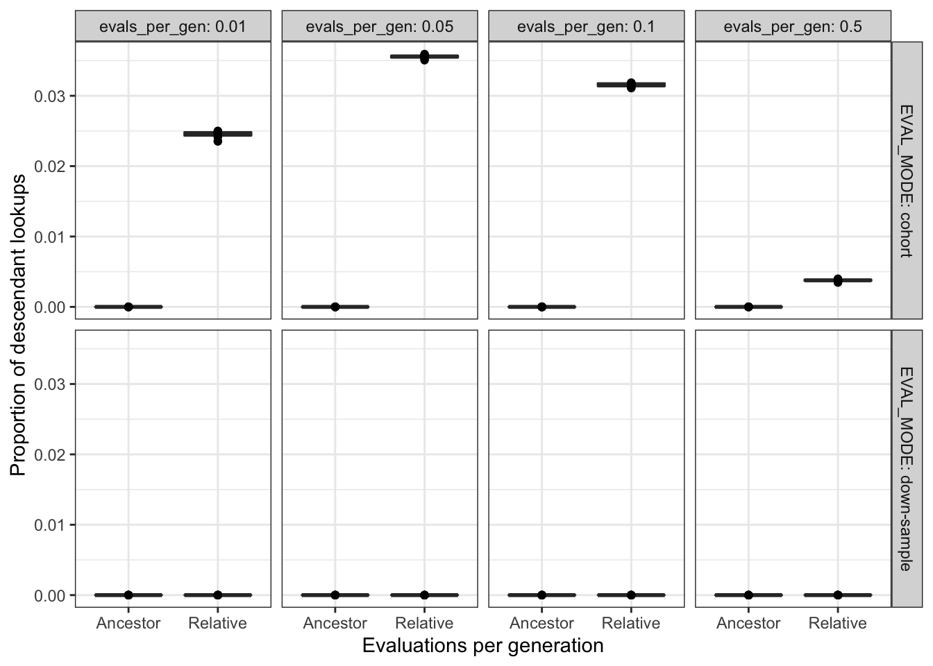

ggsave(
   filename=paste0(plot_directory, "explore-descendant-lookups.pdf")
)

## Saving 7 x 5 in image

est_source_data %>%
  filter(DIAGNOSTIC == "multipath-exploration") %>%
  filter(EVAL_MODE != "full" & EVAL_FIT_EST_MODE != "None") %>%
  ggplot(
      aes(
        x = EVAL_FIT_EST_MODE,
        y = prop_other_lookups
      )
    ) +
    geom_boxplot() +
    geom_point() +
    facet_grid(
      cols = vars(evals_per_gen),
      rows = vars(EVAL_MODE),
      labeller = label_both
    ) +
    scale_y_continuous("Proportion of other lookups") +
    scale_x_discrete("Evaluations per generation") +
    theme_bw() +
    theme(legend.position = "none")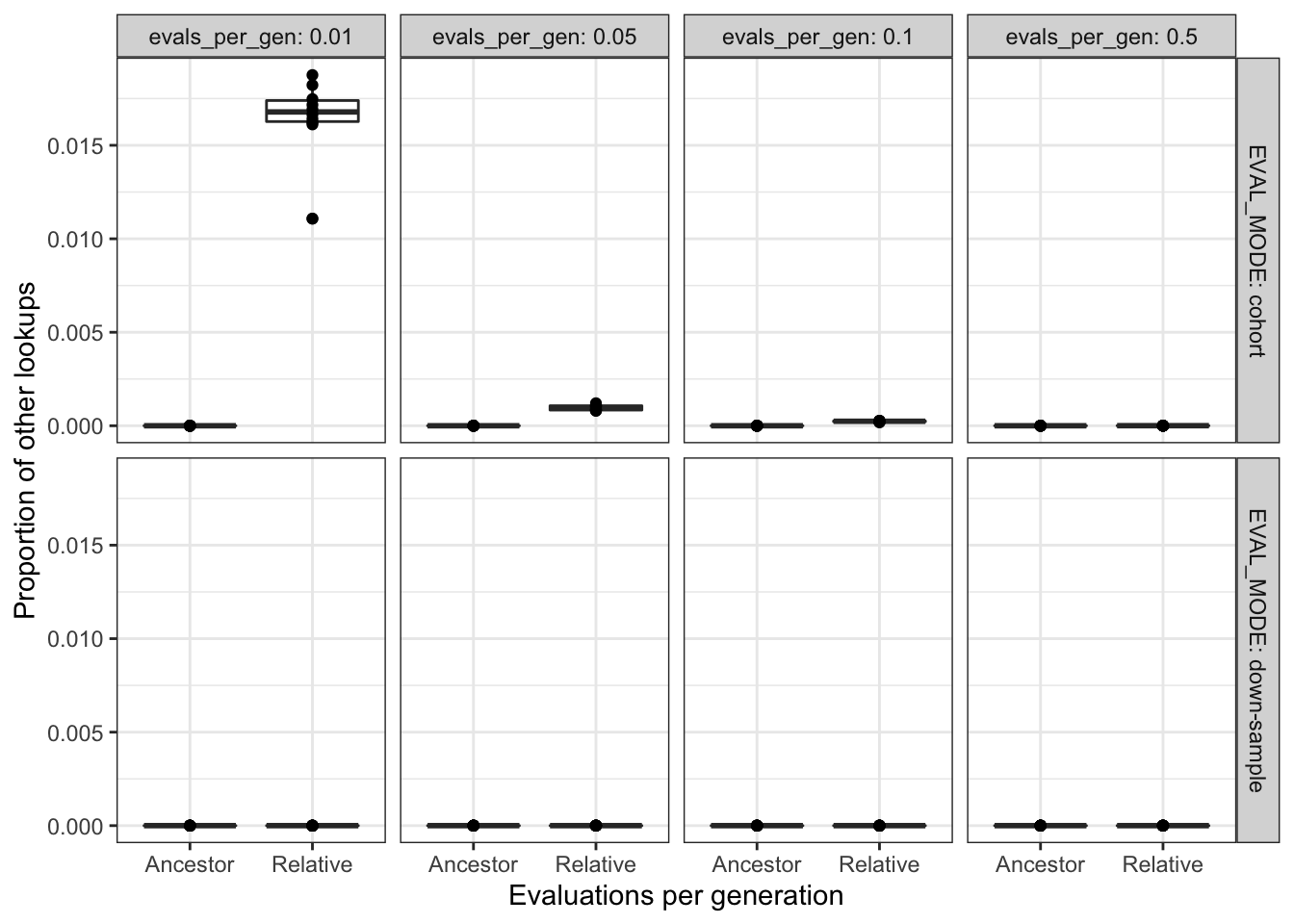

ggsave(
   filename=paste0(plot_directory, "explore-other-lookups.pdf")
)

## Saving 7 x 5 in image

est_source_data %>%
  filter(DIAGNOSTIC == "multipath-exploration") %>%
  filter(EVAL_MODE != "full" & EVAL_FIT_EST_MODE != "None") %>%
  ggplot(
      aes(
        x = EVAL_FIT_EST_MODE,
        y = prop_outside_lookups
      )
    ) +
    geom_boxplot() +
    geom_point() +
    facet_grid(
      cols = vars(evals_per_gen),
      rows = vars(EVAL_MODE),
      labeller = label_both
    ) +
    scale_y_continuous("Proportion of outside lookups") +
    scale_x_discrete("Evaluations per generation") +
    theme_bw() +
    theme(legend.position = "none")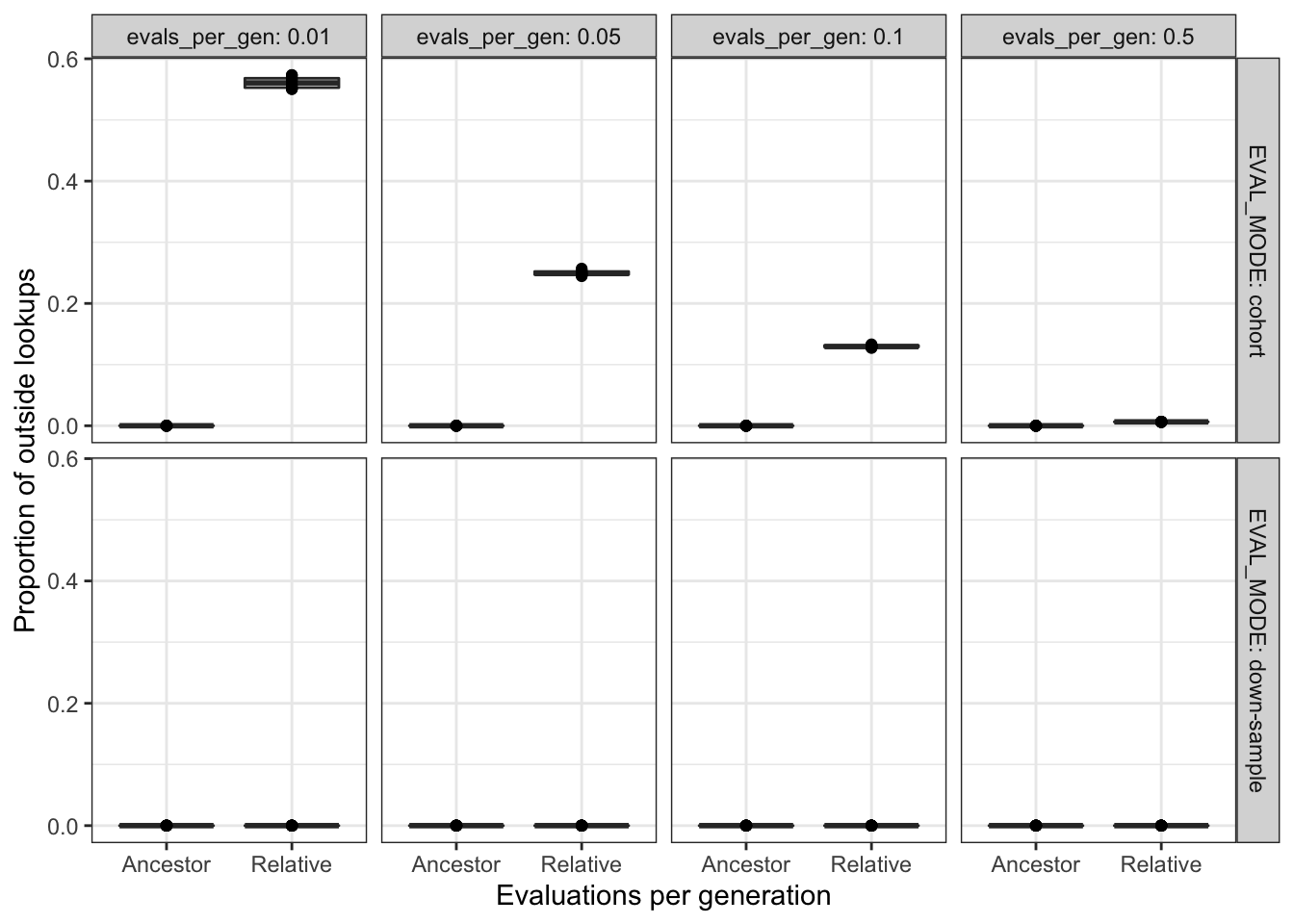

ggsave(
   filename=paste0(plot_directory, "explore-outside-lookups.pdf")
)

## Saving 7 x 5 in image

4.5 Manuscript figures

full_median_size = 1.5

subsample_labeller <- function(subsample_level) {
  return(paste("Subsample level:", subsample_level))
}

4.5.1 Contradictory objectives

Build plot panels (1 cohort, 1 down-sample)

build_con_obj_plot <- function(eval_mode) {

  full_median <- median(
    filter(
      con_obj_summary_data,
      eval_mode_row == eval_mode & EVAL_MODE == "full"
    )$pop_optimal_trait_coverage
  )

  p <- con_obj_summary_data %>%
    filter(eval_mode_row == eval_mode & EVAL_MODE != "full") %>%
    ggplot(
      aes(
        x = EVAL_FIT_EST_MODE,
        y = pop_optimal_trait_coverage,
        fill = EVAL_FIT_EST_MODE
      )
    ) +
    geom_hline(
      yintercept = full_median,
      size = full_median_size,
      alpha = 0.7,
      color = "black"
    ) +
    geom_flat_violin(
      position = position_nudge(x = .2, y = 0),
      alpha = .8,
      adjust=1.5
    ) +
    geom_point(
      mapping=aes(color=EVAL_FIT_EST_MODE),
      position = position_jitter(width = .15),
      size = .5,
      alpha = 0.8
    ) +
    geom_boxplot(
      width = .1,
      outlier.shape = NA,
      alpha = 0.5
    ) +
    scale_y_continuous(
      limits = c(-0.5, 50)
    ) +
    scale_fill_bright() +
    scale_color_bright() +
    facet_wrap(
    ~ evals_per_gen,
    nrow = 1,
    labeller = as_labeller(
      subsample_labeller
    )
    ) +
    labs(
      x = "Estimation mode",
      y = "Satisfactory trait coverage"
    ) +
    theme(
      legend.position = "none",
      axis.text.x = element_text(
        angle = 30,
        hjust = 1
      ),
      panel.border = element_rect(color="gray", size=2)
    )

  return(p)
}

con_obj_ds_plot <- build_con_obj_plot("down-sample")
con_obj_cohort_plot <- build_con_obj_plot("cohort")

Combine panels into single plot.

# Joint title: https://wilkelab.org/cowplot/articles/plot_grid.html
con_obj_title <- ggdraw() +
  draw_label(
    "Contradictory objectives diagnostic",
    fontface = 'bold',
    x = 0,
    hjust = 0
  ) +
  theme(
    # add margin on the left of the drawing canvas,
    # so title is aligned with left edge of first plot
    plot.margin = margin(0, 0, 0, 7)
  )

con_obj_grid <- plot_grid(
  con_obj_title,
  con_obj_ds_plot +
    labs(
      title = "Down-sampled lexicase"
    ) +
    theme(axis.title.x = element_blank()),
  con_obj_cohort_plot +
    labs(
      title = "Cohort lexicase"
    ),
  nrow = 3,
  ncol = 1,
  # align = "h",
  labels = c("", "a", "b"),
  rel_heights = c(0.075, 1, 1)
)
con_obj_grid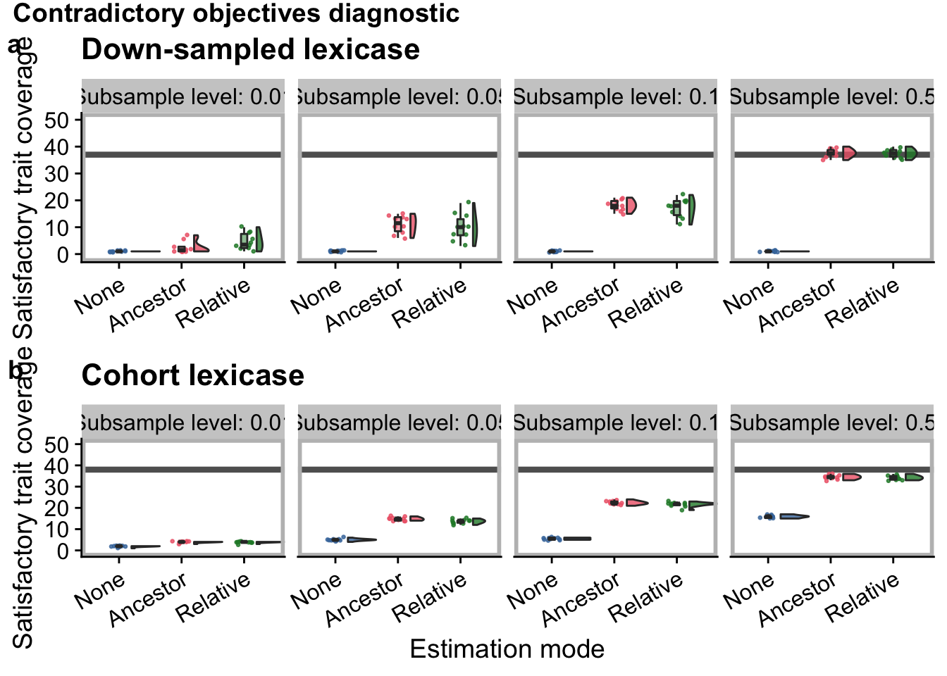

save_plot(
  filename = paste0(plot_directory, "2023-05-10-diagnostics-con-obj-final-fig.pdf"),
  plot = con_obj_grid,
  base_width = 10,
  base_height = 8,
  dpi = 600
)

4.5.2 Multi-path exploration

build_explore_plot <- function(eval_mode) {

  full_median <- median(
    filter(
      explore_summary_data,
      eval_mode_row == eval_mode & EVAL_MODE == "full"
    )$max_agg_score
  )

  p <- explore_summary_data %>%
    filter(eval_mode_row == eval_mode & EVAL_MODE != "full") %>%
    ggplot(
      aes(
        x = EVAL_FIT_EST_MODE,
        y = max_agg_score,
        fill = EVAL_FIT_EST_MODE
      )
    ) +
    geom_hline(
      yintercept = full_median,
      size = full_median_size,
      alpha = 0.7,
      color = "black"
    ) +
    geom_flat_violin(
      position = position_nudge(x = .2, y = 0),
      alpha = .8,
      adjust=1.5
    ) +
    geom_point(
      mapping=aes(color=EVAL_FIT_EST_MODE),
      position = position_jitter(width = .15),
      size = .5,
      alpha = 0.8
    ) +
    geom_boxplot(
      width = .1,
      outlier.shape = NA,
      alpha = 0.5
    ) +
    scale_y_continuous(
      limits = c(-0.5, 10005)
    ) +
    scale_fill_bright() +
    scale_color_bright() +
    facet_wrap(
    ~ evals_per_gen,
    nrow = 1,
    labeller = as_labeller(
      subsample_labeller
    )
    ) +
    labs(
      x = "Estimation mode",
      y = "Max aggregate score"
    ) +
    theme(
      legend.position = "none",
      axis.text.x = element_text(
        angle = 30,
        hjust = 1
      ),
      panel.border = element_rect(color="gray", size=2)
    )

  return(p)
}

explore_ds_plot <- build_explore_plot("down-sample")
explore_cohort_plot <- build_explore_plot("cohort")

explore_ds_plot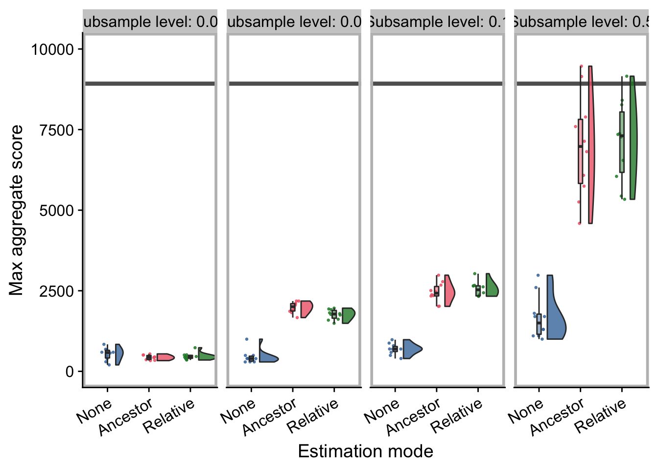

explore_cohort_plot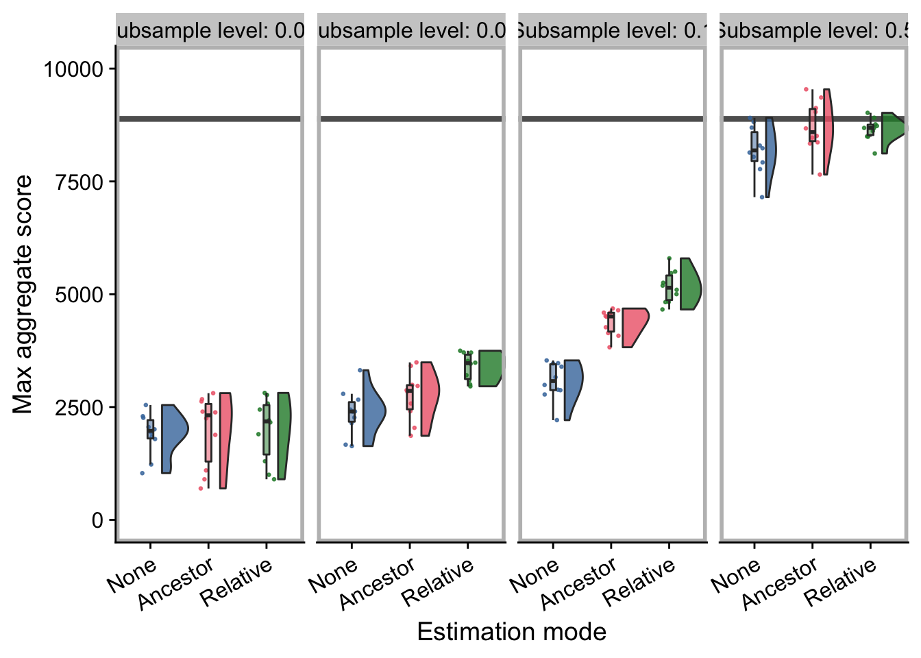

Combine panels into single plot.

# Joint title: https://wilkelab.org/cowplot/articles/plot_grid.html
explore_title <- ggdraw() +
  draw_label(
    "Multi-path exploration diagnostic",
    fontface = 'bold',
    x = 0,
    hjust = 0
  ) +
  theme(
    # add margin on the left of the drawing canvas,
    # so title is aligned with left edge of first plot
    plot.margin = margin(0, 0, 0, 7)
  )

explore_grid <- plot_grid(
  explore_title,
  explore_ds_plot +
    labs(
      title = "Down-sampled lexicase"
    ) +
    theme(axis.title.x = element_blank()),
  explore_cohort_plot +
    labs(
      title = "Cohort lexicase"
    ),
  nrow = 3,
  ncol = 1,
  # align = "h",
  labels = c("", "a", "b"),
  rel_heights = c(0.075, 1, 1)
)
explore_grid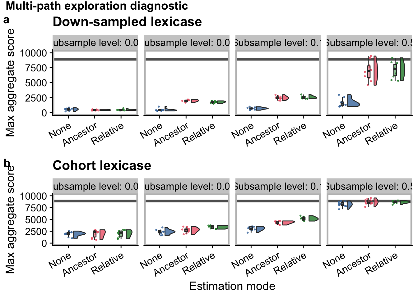

save_plot(
  filename = paste0(plot_directory, "2023-05-10-diagnostics-explore-final-fig.pdf"),
  plot = explore_grid,
  base_width = 10,
  base_height = 8,
  dpi = 600
)