Chapter 8 Graph property correlations
We screened for graph properties correlated with community transitionability scores.
8.1 Dependencies and setup
library(tidyverse)
library(Hmisc)
library(broom)
library(knitr)
library(kableExtra)
# Check if Rmd is being compiled using bookdown
bookdown <- exists("bookdown_build")experiment_slug <- "2024-03-08-varied-interaction-matrices"
working_directory <- paste(
"experiments",
experiment_slug,
"analysis",
sep = "/"
)
# Adjust working directory if being knitted for bookdown build.
if (bookdown) {
working_directory <- paste0(
bookdown_wd_prefix,
working_directory
)
}
plot_dir <- paste(
working_directory,
"plots",
sep = "/"
)
data_path <- paste(
working_directory,
"data",
"world_summary_final_update_with-graph-props.csv",
sep = "/"
)
data <- read_csv(data_path)Set cowplot theme as default plotting theme.
theme_set(theme_cowplot())8.2 Data preprocessing
max_update <- max(data$update)
# Ensure that we just have measurements from final update.
data <- data %>%
  filter(update == max_update) %>%
  mutate(
    interaction_matrix = as.factor(interaction_matrix),
    graph_type = as.factor(graph_type),
    summary_mode = as.factor(summary_mode),
    update = as.numeric(update),
    SEED = as.factor(SEED),
    graph_file = str_split_i(DIFFUSION_SPATIAL_STRUCTURE_FILE, "/", -1)
  ) %>%
  mutate(
    graph_file = as.factor(graph_file)
  )
# write_csv(
#   data,
#   "world_summary_final_update.csv"
# )

# For each row, assign graph properties
properties <- c(
  "graph_prop_density",
  "graph_prop_degree_mean",
  "graph_prop_degree_median",
  "graph_prop_degree_variance",
  "graph_prop_girth",
  "graph_prop_degree_assortivity_coef",
  "graph_prop_num_bridges",
  "graph_prop_max_clique_size",
  "graph_prop_transitivity",
  "graph_prop_avg_clustering",
  "graph_prop_num_connected_components",
  "graph_prop_num_articulation_points",
  "graph_prop_avg_node_connectivity",
  "graph_prop_edge_connectivity",
  "graph_prop_node_connectivity",
  "graph_prop_diameter",
  "graph_prop_radius",
  "graph_prop_kemeny_constant",
  "graph_prop_global_efficiency",
  "graph_prop_wiener_index",
  "graph_prop_longest_shortest_path"
)

# (3) Pivot longer
long_data <- data %>%
  mutate(
    graph_prop_diameter = case_when(
      graph_prop_diameter == "error" ~ "-1",
      .default = graph_prop_diameter
    ),
    graph_prop_radius = case_when(
      graph_prop_radius == "error" ~ "-1",
      .default = graph_prop_radius
    ),
    graph_prop_kemeny_constant = case_when(
      graph_prop_kemeny_constant == "error" ~ "-1",
      .default = graph_prop_kemeny_constant
    )
  ) %>%
  mutate(
    graph_prop_diameter = as.numeric(graph_prop_diameter),
    graph_prop_radius = as.numeric(graph_prop_radius),
    graph_prop_kemeny_constant = as.numeric(graph_prop_kemeny_constant)
  ) %>%
  select(
    !c(
      DIFFUSION_SPATIAL_STRUCTURE_FILE,
      GROUP_REPRO_SPATIAL_STRUCTURE_FILE,
      INTERACTION_SOURCE
    )
  ) %>%
  filter(
    summary_mode == "ranked_threshold"
  ) %>%
  pivot_longer(
    cols = properties,
    names_to = "graph_property",
    values_to = "graph_property_value"
  ) %>%
  filter(
    (!is.na(graph_property_value)) & graph_property_value != "Inf" &
    (!(graph_property == "graph_prop_diameter" & (graph_property_value == "-1"))) &
    (!(graph_property == "graph_prop_radius" & (graph_property_value == "-1"))) &
    (!(graph_property == "graph_prop_kemeny_constant" & (graph_property_value == "-1")))
  ) %>%
  mutate(
    graph_property_value = as.numeric(graph_property_value),
    graph_property = str_remove(graph_property, "graph_prop_")
  ) %>%
  mutate(
    graph_property = as.factor(graph_property)
  )
# write_csv(long_data, "test.csv")
8.3 Plot relationships between transitionability and graph properties
rel_plot <- long_data %>%
  ggplot(
    aes(
      x = graph_property_value,
      y = logged_mult_score
    )
  ) +
  geom_point(aes(color = graph_type)) +
  geom_smooth(
    method = "lm",
    color = "black"
  ) +
  facet_grid(
    interaction_matrix ~ graph_property,
    scales = "free"
  )

rel_plot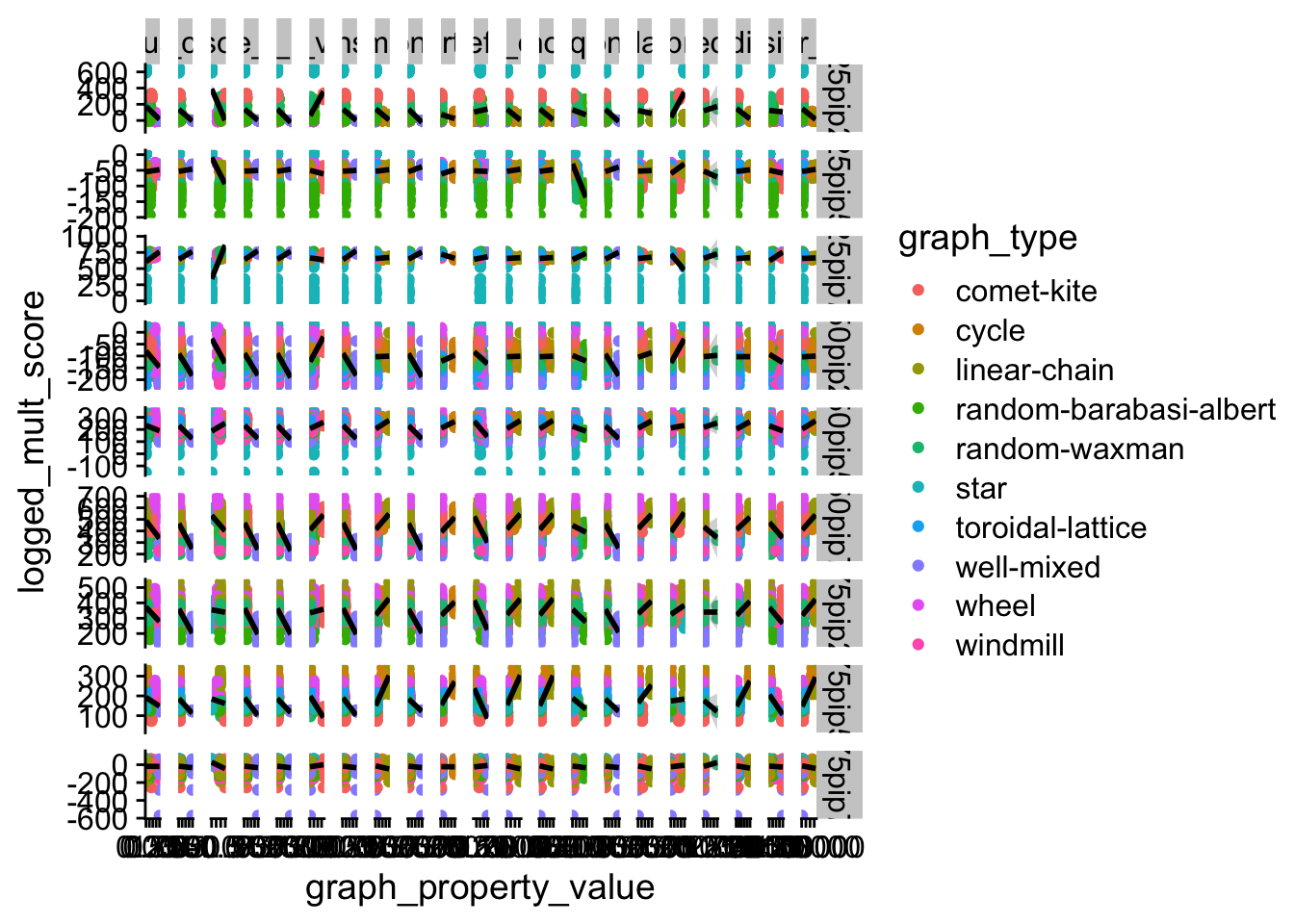
ggsave(
  plot = rel_plot,
  filename = paste(
    plot_dir,
    "property_relationships.pdf",
    sep = "/"
  ),
  width = 40,
  height = 20
)
8.4 Measure correlations
# Reference for running correlations over tidy data:
# https://dominicroye.github.io/en/2019/tidy-correlation-tests-in-r/
cor_fun <- function(data) {
  cor.test(
    data$graph_property_value,
    data$logged_mult_score,
    method = "spearman",
    exact = FALSE
  ) %>% tidy()
}

nested <- long_data %>%
  select(
    c(
      interaction_matrix,
      graph_property,
      graph_property_value,
      logged_mult_score
    )
  ) %>%
  group_by(interaction_matrix, graph_property) %>%
  nest() %>%
  mutate(
    model = map(data, cor_fun)
  )

full_corr <- select(nested, -data) %>% unnest()
full_corr <- full_corr %>%
  mutate(
    abs_estimate = abs(estimate)
  ) %>%
  arrange(
    desc(abs_estimate)
  ) %>%
  group_by(
    interaction_matrix
  ) %>%
  mutate(
    p.value.adj = p.adjust(p.value, method = "holm")
  ) %>%
  filter(
    p.value.adj <= 0.05
  )

full_corr_table <- kable(full_corr) %>%
  kable_styling(latex_options = "striped")
save_kable(
  full_corr_table,
  paste(
    plot_dir,
    "correlation_table.pdf",
    sep = "/"
  )
)
8.4.1 Top three significant correlations per interaction matrix
Break correlations down by interaction matrix
interaction_matrices <- levels(long_data$interaction_matrix)
for (mat_type in interaction_matrices) {
mat_data <- filter(long_data, interaction_matrix == mat_type)
nested <- mat_data %>%
select(
c(
interaction_matrix,
graph_property,
graph_property_value,
logged_mult_score
)
) %>%
group_by(interaction_matrix, graph_property) %>%
nest() %>%
mutate(
model = map(data, cor_fun)
)
im_corr <- select(nested, -data) %>% unnest()
im_corr <- im_corr %>%
mutate(
abs_estimate = abs(estimate)
) %>%
arrange(
desc(abs_estimate)
) %>%
ungroup() %>%
group_by(
interaction_matrix
) %>%
mutate(
p.value.adj = p.adjust(p.value, method = "holm")
) %>%
filter(
p.value.adj < 0.05
)
im_corr_table <- kable(im_corr) %>%
kable_styling(latex_options = "striped")
save_kable(
im_corr_table,
paste(
plot_dir,
paste0("correlation_table_", mat_type, ".pdf"),
sep = "/"
)
)
top_corr <- im_corr %>%
slice_max(
abs_estimate,
n = 3
)
top_corr_table <- kable(top_corr) %>%
kable_styling(latex_options = "striped")
save_kable(
top_corr_table,
paste(
plot_dir,
paste0("t3_correlation_table_", mat_type, ".pdf"),
sep = "/"
)
)
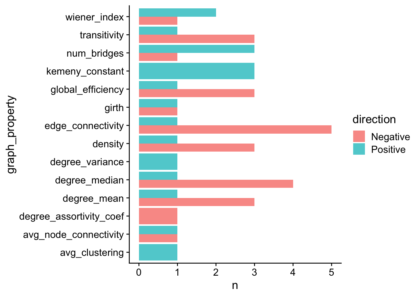
}8.4.2 Distrubition of correlations >= 0.5 strength
# Look at distribution of correlations >= 0.5 strength
corr_str_thresh <- 0.5
full_corr_thresh <- full_corr %>%
  mutate(
    direction = case_when(
      estimate < 0 ~ "Negative",
      estimate >= 0 ~ "Positive"
    )
  ) %>%
  mutate(
    direction = as.factor(direction)
  ) %>%
  filter(abs_estimate >= corr_str_thresh & p.value.adj <= 0.05)

corr_counts <- full_corr_thresh %>%
  dplyr::group_by(graph_property, direction) %>%
  dplyr::summarize(
    n = n()
  )

# If something has one direction, but not other, fill in 0 for other.
# For property in properties
correlation_dirs_plot <- corr_counts %>%
  ggplot(
    aes(
      x = graph_property,
      fill = direction,
      y = n
    )
  ) +
  geom_bar(stat = "identity", position = position_dodge(), alpha = 0.75) +
  coord_flip()

ggsave(
  plot = correlation_dirs_plot,
  filename = paste(
    plot_dir,
    "most_moderate_correlations.pdf",
    sep = "/"
  )
)
correlation_dirs_plot