Chapter 7 Avida - Squished lattice experiment analyses
7.1 Dependencies and setup
library(tidyverse)
library(cowplot)
library(RColorBrewer)
library(khroma)
library(rstatix)
library(knitr)
library(kableExtra)
source("https://gist.githubusercontent.com/benmarwick/2a1bb0133ff568cbe28d/raw/fb53bd97121f7f9ce947837ef1a4c65a73bffb3f/geom_flat_violin.R")
# Check if Rmd is being compiled using bookdown
bookdown <- exists("bookdown_build")experiment_slug <- "2025-04-17-squished-lattice-longer"
working_directory <- paste(
"experiments",
experiment_slug,
"analysis",
sep = "/"
)
# Adjust working directory if being knitted for bookdown build.
if (bookdown) {
working_directory <- paste0(
bookdown_wd_prefix,
working_directory
)
}# Configure our default graphing theme
theme_set(theme_cowplot())
# Create a directory to store plots
plot_dir <- paste(
working_directory,
"plots",
sep = "/"
)
dir.create(
plot_dir,
showWarnings = FALSE
)focal_graphs <- c(
"toroidal-lattice_60x60",
"toroidal-lattice_15x240",
"toroidal-lattice_2x1800",
"cycle"
)
# Load summary data from final update
data_path <- paste(
working_directory,
"data",
"summary.csv",
sep = "/"
)
data <- read_csv(data_path)
data <- data %>%
filter(graph_type %in% focal_graphs) %>%
mutate(
graph_type = factor(
graph_type,
levels = focal_graphs
),
ENVIRONMENT_FILE = as.factor(ENVIRONMENT_FILE)
)time_series_path <- paste(
working_directory,
"data",
"time_series.csv",
sep = "/"
)
time_series_data <- read_csv(time_series_path)
time_series_data <- time_series_data %>%
filter(graph_type %in% focal_graphs) %>%
mutate(
graph_type = factor(
graph_type,
levels = focal_graphs
),
ENVIRONMENT_FILE = as.factor(ENVIRONMENT_FILE),
seed = as.factor(seed)
)
time_series_data <- time_series_data %>% filter(seed %in% data$seed)# Check that all runs completed
data %>%
filter(update == 400000) %>%
group_by(graph_type) %>%
summarize(
n = n()
)## # A tibble: 4 × 2
## graph_type n
## <fct> <int>
## 1 toroidal-lattice_60x60 50
## 2 toroidal-lattice_15x240 50
## 3 toroidal-lattice_2x1800 50
## 4 cycle 507.2 Number of tasks completed
pop_tasks_total_plt <- ggplot(
  data = data,
  mapping = aes(
    x = graph_type,
    y = pop_task_total,
    fill = graph_type
  )
) +
  geom_flat_violin(
    position = position_nudge(x = .2, y = 0),
    alpha = .8
  ) +
  geom_point(
    mapping=aes(color = graph_type),
    position = position_jitter(width = .15),
    size = .5,
    alpha = 0.8
  ) +
  geom_boxplot(
    width = .1,
    outlier.shape = NA,
    alpha = 0.5
  ) +
  theme(
    legend.position = "none",
    axis.text.x = element_text(
      angle = 30,
      hjust = 1
    )
  )

ggsave(
  filename = paste0(plot_dir, "/pop_tasks_total.pdf"),
  plot = pop_tasks_total_plt,
  width = 15,
  height = 10
)

pop_tasks_total_plt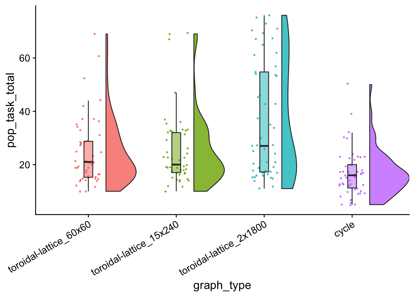
data %>%
  group_by(graph_type) %>%
  summarize(
    reps = n(),
    median_pop_tasks = median(pop_task_total),
    mean_pop_tasks = mean(pop_task_total)
  ) %>%
  arrange(
    desc(mean_pop_tasks)
  )
## # A tibble: 4 × 4
## graph_type reps median_pop_tasks mean_pop_tasks
## <fct> <int> <dbl> <dbl>
## 1 toroidal-lattice_2x1800 50 27 36.6
## 2 toroidal-lattice_15x240 50 20 25.2
## 3 toroidal-lattice_60x60 50 21 24.6
## 4 cycle 50 16 16.7kruskal.test(
formula = pop_task_total ~ graph_type,
data = data
)##
## Kruskal-Wallis rank sum test
##
## data: pop_task_total by graph_type
## Kruskal-Wallis chi-squared = 34.696, df = 3, p-value = 1.412e-07wc_results <- pairwise.wilcox.test(
x = data$pop_task_total,
g = data$graph_type,
p.adjust.method = "holm",
exact = FALSE
)
pop_task_wc_table <- kbl(wc_results$p.value) %>% kable_styling()
save_kable(pop_task_wc_table, paste0(plot_dir, "/pop_task_wc_table.pdf"))
pop_task_wc_table| toroidal-lattice_60x60 | toroidal-lattice_15x240 | toroidal-lattice_2x1800 | |
|---|---|---|---|
| toroidal-lattice_15x240 | 0.9011082 | NA | NA |
| toroidal-lattice_2x1800 | 0.0313929 | 0.0386732 | NA |
| cycle | 0.0010892 | 0.0002773 | 8e-07 |
7.3 Dominant tasks
dom_tasks_total_plt <- ggplot(
  data = data,
  mapping = aes(
    x = graph_type,
    y = dom_task_total,
    fill = graph_type
  )
) +
  geom_flat_violin(
    position = position_nudge(x = .2, y = 0),
    alpha = .8
  ) +
  geom_point(
    mapping=aes(color = graph_type),
    position = position_jitter(width = .15),
    size = .5,
    alpha = 0.8
  ) +
  geom_boxplot(
    width = .1,
    outlier.shape = NA,
    alpha = 0.5
  ) +
  theme(
    legend.position = "none",
    axis.text.x = element_text(
      angle = 30,
      hjust = 1
    )
  )

ggsave(
  filename = paste0(plot_dir, "/dom_tasks_total.pdf"),
  plot = dom_tasks_total_plt,
  width = 15,
  height = 10
)

dom_tasks_total_plt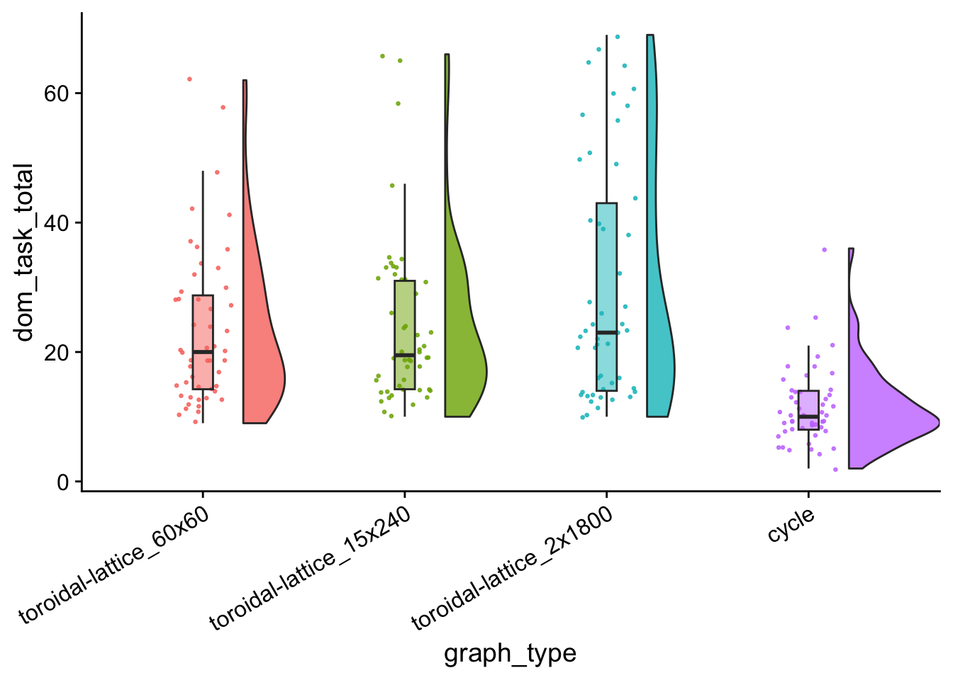
data %>%
  group_by(graph_type) %>%
  summarize(
    reps = n(),
    median_dom_task_total = median(dom_task_total),
    mean_dom_task_total = mean(dom_task_total)
  ) %>%
  arrange(
    desc(mean_dom_task_total)
  )
## # A tibble: 4 × 4
## graph_type reps median_dom_task_total mean_dom_task_total
## <fct> <int> <dbl> <dbl>
## 1 toroidal-lattice_2x1800 50 23 30.1
## 2 toroidal-lattice_15x240 50 19.5 24.1
## 3 toroidal-lattice_60x60 50 20 23.5
## 4 cycle 50 10 11.5kruskal.test(
formula = dom_task_total ~ graph_type,
data = data
)##
## Kruskal-Wallis rank sum test
##
## data: dom_task_total by graph_type
## Kruskal-Wallis chi-squared = 62.705, df = 3, p-value = 1.553e-13wc_results <- pairwise.wilcox.test(
x = data$dom_task_total,
g = data$graph_type,
p.adjust.method = "holm",
exact = FALSE
)
dom_task_total_wc_table <- kbl(wc_results$p.value) %>% kable_styling()
save_kable(dom_task_total_wc_table, paste0(plot_dir, "/dom_task_total_wc_table.pdf"))
dom_task_total_wc_table| toroidal-lattice_60x60 | toroidal-lattice_15x240 | toroidal-lattice_2x1800 | |
|---|---|---|---|
| toroidal-lattice_15x240 | 0.8224738 | NA | NA |
| toroidal-lattice_2x1800 | 0.4960864 | 0.5387756 | NA |
| cycle | 0.0000000 | 0.0000000 | 0 |
Tasks done by organisms not in dominant taxon:
data <- data %>%
  mutate(
    nondom_pop_task_prop = case_when(
      pop_task_total == 0 ~ 0,
      .default = (pop_task_total - dom_task_total) / (pop_task_total)
    )
  )
nondom_tasks_total_plt <- ggplot(
    data = data,
    mapping = aes(
      x = graph_type,
      y = nondom_pop_task_prop,
      fill = graph_type
    )
  ) +
  geom_flat_violin(
    position = position_nudge(x = .2, y = 0),
    alpha = .8
  ) +
  geom_point(
    mapping=aes(color = graph_type),
    position = position_jitter(width = .15),
    size = .5,
    alpha = 0.8
  ) +
  geom_boxplot(
    width = .1,
    outlier.shape = NA,
    alpha = 0.5
  ) +
  theme(
    legend.position = "none",
    axis.text.x = element_text(
      angle = 30,
      hjust = 1
    )
  )

ggsave(
  filename = paste0(plot_dir, "/non_dom_tasks_total.pdf"),
  plot = nondom_tasks_total_plt,
  width = 15,
  height = 10
)

nondom_tasks_total_plt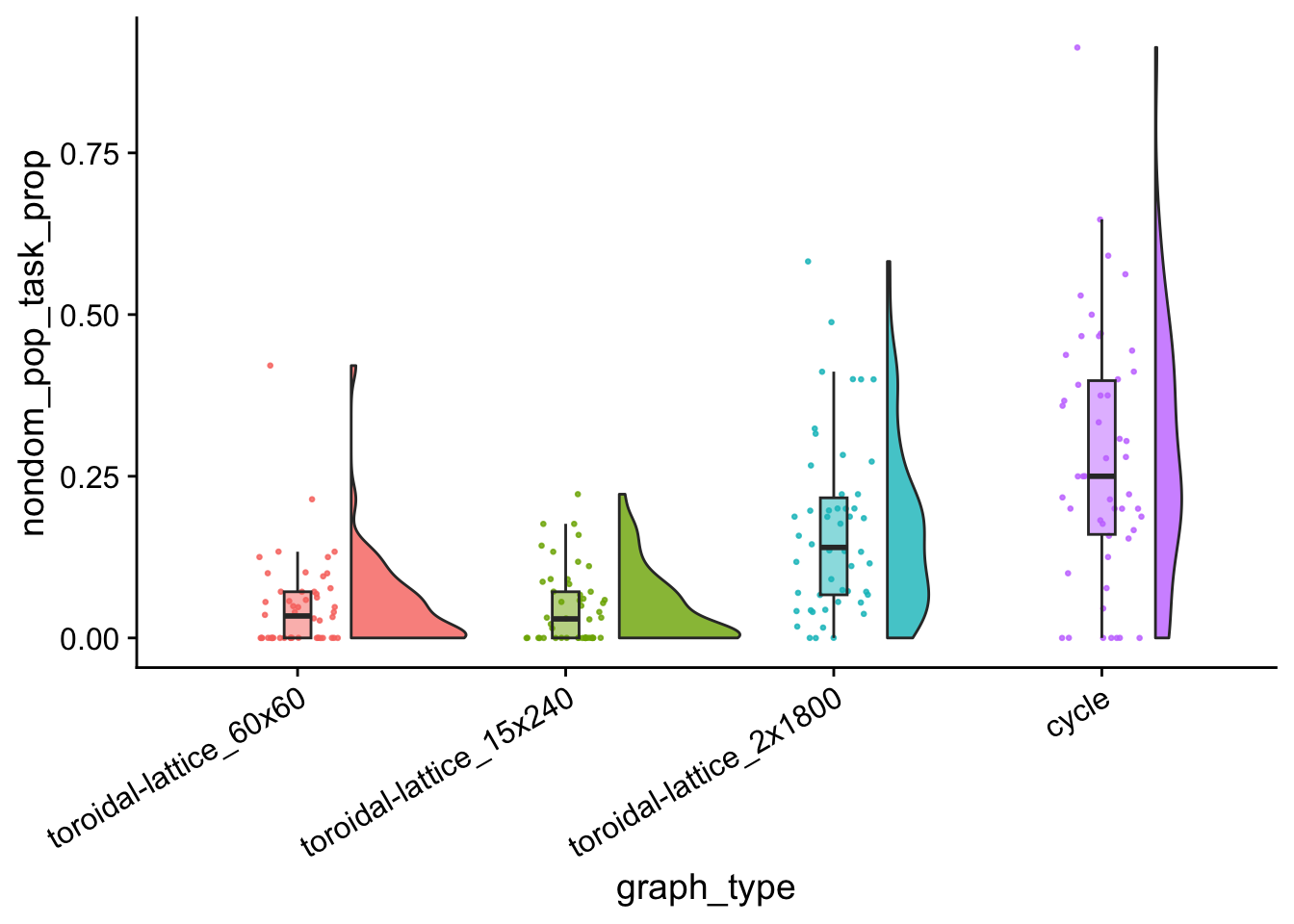
data %>%
  group_by(graph_type) %>%
  summarize(
    reps = n(),
    median_nondom_pop_task_prop = median(nondom_pop_task_prop),
    mean_nondom_pop_task_prop = mean(nondom_pop_task_prop)
  ) %>%
  arrange(
    desc(mean_nondom_pop_task_prop)
  )
## # A tibble: 4 × 4
## graph_type reps median_nondom_pop_task_…¹ mean_nondom_pop_task…²
## <fct> <int> <dbl> <dbl>
## 1 cycle 50 0.25 0.276
## 2 toroidal-lattice_2x1800 50 0.140 0.168
## 3 toroidal-lattice_60x60 50 0.0340 0.0498
## 4 toroidal-lattice_15x240 50 0.0294 0.0467
## # ℹ abbreviated names: ¹median_nondom_pop_task_prop, ²mean_nondom_pop_task_propkruskal.test(
formula = nondom_pop_task_prop ~ graph_type,
data = data
)##
## Kruskal-Wallis rank sum test
##
## data: nondom_pop_task_prop by graph_type
## Kruskal-Wallis chi-squared = 72.727, df = 3, p-value = 1.112e-15wc_results <- pairwise.wilcox.test(
x = data$nondom_pop_task_prop,
g = data$graph_type,
p.adjust.method = "holm",
exact = FALSE
)
nondom_pop_task_prop_wc_table <- kbl(wc_results$p.value) %>% kable_styling()
save_kable(nondom_pop_task_prop_wc_table, paste0(plot_dir, "/nondom_pop_task_prop_wc_table.pdf"))
nondom_pop_task_prop_wc_table| toroidal-lattice_60x60 | toroidal-lattice_15x240 | toroidal-lattice_2x1800 | |
|---|---|---|---|
| toroidal-lattice_15x240 | 0.9884975 | NA | NA |
| toroidal-lattice_2x1800 | 0.0000002 | 2e-07 | NA |
| cycle | 0.0000000 | 0e+00 | 0.0066588 |
7.4 Dominant gestation time
dom_gestation_time_plt <- ggplot(
    data = data,
    mapping = aes(
      x = graph_type,
      y = dom_detail_gestation_time,
      fill = graph_type
    )
  ) +
  geom_flat_violin(
    position = position_nudge(x = .2, y = 0),
    alpha = .8
  ) +
  geom_point(
    mapping=aes(color = graph_type),
    position = position_jitter(width = .15),
    size = .5,
    alpha = 0.8
  ) +
  geom_boxplot(
    width = .1,
    outlier.shape = NA,
    alpha = 0.5
  ) +
  theme(
    legend.position = "none",
    axis.text.x = element_text(
      angle = 30,
      hjust = 1
    )
  )

ggsave(
  filename = paste0(plot_dir, "/dom_gestation_time.pdf"),
  plot = dom_gestation_time_plt,
  width = 15,
  height = 10
)

dom_gestation_time_plt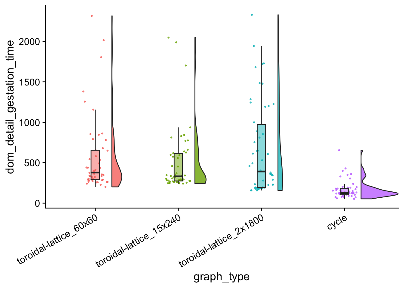
data %>%
  group_by(graph_type) %>%
  summarize(
    reps = n(),
    median_dom_detail_gestation_time = median(dom_detail_gestation_time),
    mean_dom_detail_gestation_time = mean(dom_detail_gestation_time)
  ) %>%
  arrange(
    desc(mean_dom_detail_gestation_time)
  )
## # A tibble: 4 × 4
## graph_type reps median_dom_detail_gesta…¹ mean_dom_detail_gest…²
## <fct> <int> <dbl> <dbl>
## 1 toroidal-lattice_2x1800 50 392. 660.
## 2 toroidal-lattice_60x60 50 378 569.
## 3 toroidal-lattice_15x240 50 332. 508.
## 4 cycle 50 126. 166.
## # ℹ abbreviated names: ¹median_dom_detail_gestation_time,
## # ²mean_dom_detail_gestation_timekruskal.test(
formula = dom_detail_gestation_time ~ graph_type,
data = data
)##
## Kruskal-Wallis rank sum test
##
## data: dom_detail_gestation_time by graph_type
## Kruskal-Wallis chi-squared = 77.537, df = 3, p-value < 2.2e-16wc_results <- pairwise.wilcox.test(
x = data$dom_detail_gestation_time,
g = data$graph_type,
p.adjust.method = "holm",
exact = FALSE
)
dom_detail_gestation_time_wc_table <- kbl(wc_results$p.value) %>% kable_styling()
save_kable(dom_detail_gestation_time_wc_table, paste0(plot_dir, "/dom_detail_gestation_time_wc_table.pdf"))
dom_detail_gestation_time_wc_table| toroidal-lattice_60x60 | toroidal-lattice_15x240 | toroidal-lattice_2x1800 | |
|---|---|---|---|
| toroidal-lattice_15x240 | 0.8010941 | NA | NA |
| toroidal-lattice_2x1800 | 1.0000000 | 1 | NA |
| cycle | 0.0000000 | 0 | 0 |
7.5 Dominant genome length
dom_genome_length_plt <- ggplot(
    data = data,
    mapping = aes(
      x = graph_type,
      y = dom_detail_genome_length,
      fill = graph_type
    )
  ) +
  geom_flat_violin(
    position = position_nudge(x = .2, y = 0),
    alpha = .8
  ) +
  geom_point(
    mapping=aes(color = graph_type),
    position = position_jitter(width = .15),
    size = .5,
    alpha = 0.8
  ) +
  geom_boxplot(
    width = .1,
    outlier.shape = NA,
    alpha = 0.5
  ) +
  theme(
    legend.position = "none",
    axis.text.x = element_text(
      angle = 30,
      hjust = 1
    )
  )

ggsave(
  filename = paste0(plot_dir, "/dom_genome_length.pdf"),
  plot = dom_genome_length_plt,
  width = 15,
  height = 10
)

dom_genome_length_plt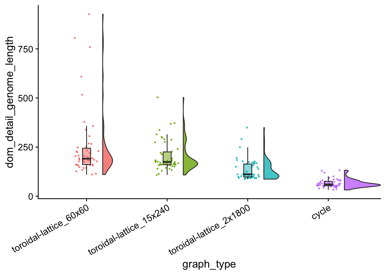
data %>%
  group_by(graph_type) %>%
  summarize(
    reps = n(),
    median_dom_detail_genome_length = median(dom_detail_genome_length),
    mean_dom_detail_genome_length = mean(dom_detail_genome_length)
  ) %>%
  arrange(
    desc(mean_dom_detail_genome_length)
  )
## # A tibble: 4 × 4
## graph_type reps median_dom_detail_genom…¹ mean_dom_detail_geno…²
## <fct> <int> <dbl> <dbl>
## 1 toroidal-lattice_60x60 50 191 252.
## 2 toroidal-lattice_15x240 50 174 203.
## 3 toroidal-lattice_2x1800 50 112. 134.
## 4 cycle 50 60 65.4
## # ℹ abbreviated names: ¹median_dom_detail_genome_length,
## # ²mean_dom_detail_genome_lengthkruskal.test(
formula = dom_detail_genome_length ~ graph_type,
data = data
)##
## Kruskal-Wallis rank sum test
##
## data: dom_detail_genome_length by graph_type
## Kruskal-Wallis chi-squared = 133.54, df = 3, p-value < 2.2e-16wc_results <- pairwise.wilcox.test(
x = data$dom_detail_genome_length,
g = data$graph_type,
p.adjust.method = "holm",
exact = FALSE
)
dom_detail_genome_length_wc_table <- kbl(wc_results$p.value) %>% kable_styling()
save_kable(dom_detail_genome_length_wc_table, paste0(plot_dir, "/dom_detail_genome_length_wc_table.pdf"))
dom_detail_genome_length_wc_table| toroidal-lattice_60x60 | toroidal-lattice_15x240 | toroidal-lattice_2x1800 | |
|---|---|---|---|
| toroidal-lattice_15x240 | 0.0972676 | NA | NA |
| toroidal-lattice_2x1800 | 0.0000000 | 1e-07 | NA |
| cycle | 0.0000000 | 0e+00 | 0 |
7.6 Task profile entropy
task_profile_entropy_plt <- ggplot(
    data = data,
    mapping = aes(
      x = graph_type,
      y = task_profile_entropy,
      fill = graph_type
    )
  ) +
  geom_flat_violin(
    position = position_nudge(x = .2, y = 0),
    alpha = .8
  ) +
  geom_point(
    mapping=aes(color = graph_type),
    position = position_jitter(width = .15),
    size = .5,
    alpha = 0.8
  ) +
  geom_boxplot(
    width = .1,
    outlier.shape = NA,
    alpha = 0.5
  ) +
  theme(
    legend.position = "none",
    axis.text.x = element_text(
      angle = 30,
      hjust = 1
    )
  )

ggsave(
  filename = paste0(plot_dir, "/task_profile_entropy.pdf"),
  plot = task_profile_entropy_plt,
  width = 15,
  height = 10
)

task_profile_entropy_plt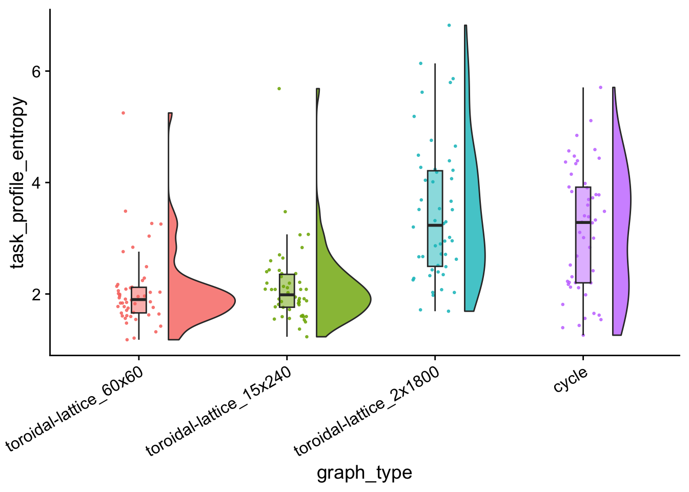
task_profile_count_plt <- ggplot(
    data = data,
    mapping = aes(
      x = graph_type,
      y = task_profile_count,
      fill = graph_type
    )
  ) +
  geom_flat_violin(
    position = position_nudge(x = .2, y = 0),
    alpha = .8
  ) +
  geom_point(
    mapping=aes(color = graph_type),
    position = position_jitter(width = .15),
    size = .5,
    alpha = 0.8
  ) +
  geom_boxplot(
    width = .1,
    outlier.shape = NA,
    alpha = 0.5
  ) +
  theme(
    legend.position = "none",
    axis.text.x = element_text(
      angle = 30,
      hjust = 1
    )
  )

ggsave(
  filename = paste0(plot_dir, "/task_profile_count.pdf"),
  plot = task_profile_count_plt,
  width = 15,
  height = 10
)

task_profile_count_plt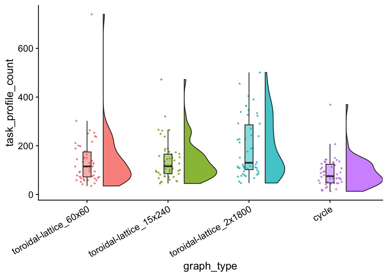
7.7 Average generation
avg_generation_plt <- ggplot(
    data = data,
    mapping = aes(
      x = graph_type,
      y = time_average_generation,
      fill = graph_type
    )
  ) +
  geom_flat_violin(
    position = position_nudge(x = .2, y = 0),
    alpha = .8
  ) +
  geom_point(
    mapping=aes(color = graph_type),
    position = position_jitter(width = .15),
    size = .5,
    alpha = 0.8
  ) +
  geom_boxplot(
    width = .1,
    outlier.shape = NA,
    alpha = 0.5
  ) +
  theme(
    legend.position = "none",
    axis.text.x = element_text(
      angle = 30,
      hjust = 1
    )
  )

ggsave(
  filename = paste0(plot_dir, "/avg_generation.pdf"),
  plot = avg_generation_plt,
  width = 15,
  height = 10
)

avg_generation_plt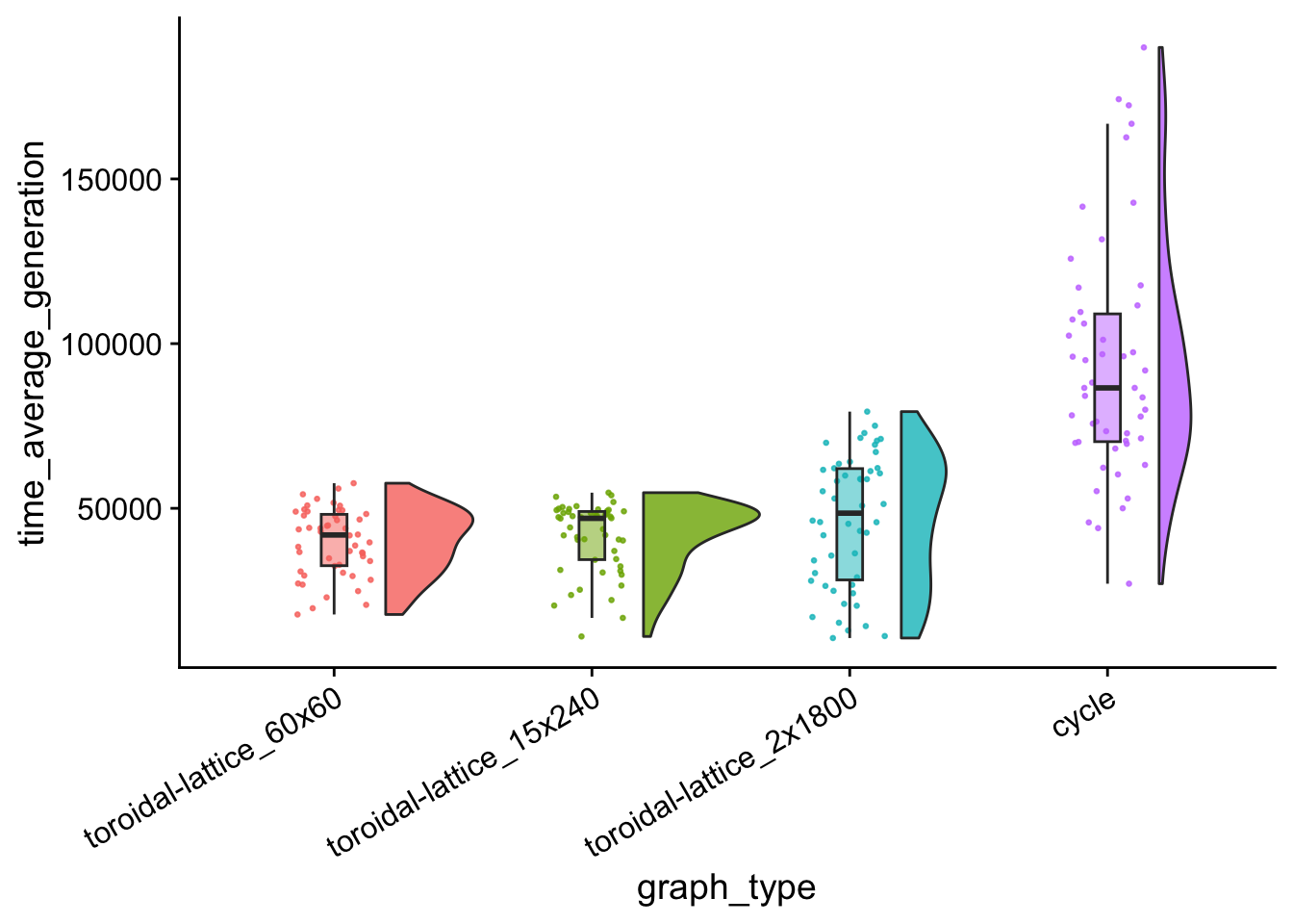
data %>%
  group_by(graph_type) %>%
  summarize(
    reps = n(),
    median_time_average_generation = median(time_average_generation),
    mean_time_average_generation = mean(time_average_generation)
  ) %>%
  arrange(
    desc(mean_time_average_generation)
  )
## # A tibble: 4 × 4
## graph_type reps median_time_average_gen…¹ mean_time_average_ge…²
## <fct> <int> <dbl> <dbl>
## 1 cycle 50 86561. 93949.
## 2 toroidal-lattice_2x1800 50 48531. 46331.
## 3 toroidal-lattice_15x240 50 46955. 41302.
## 4 toroidal-lattice_60x60 50 41905. 39813.
## # ℹ abbreviated names: ¹median_time_average_generation,
## # ²mean_time_average_generation7.8 Population task count over time
pop_task_cnt_ts <- ggplot(
    data = time_series_data,
    mapping = aes(
      x = update,
      y = pop_task_total_tasks_done,
      color = graph_type,
      fill = graph_type
    )
  ) +
  stat_summary(fun = "mean", geom = "line") +
  stat_summary(
    fun.data = "mean_cl_boot",
    fun.args = list(conf.int = 0.95),
    geom = "ribbon",
    alpha = 0.2,
    linetype = 0
  ) +
  theme(legend.position = "bottom")

ggsave(
  plot = pop_task_cnt_ts,
  filename = paste0(
    working_directory,
    "/plots/pop_tasks_ts.pdf"
  ),
  width = 15,
  height = 10
)

pop_task_cnt_ts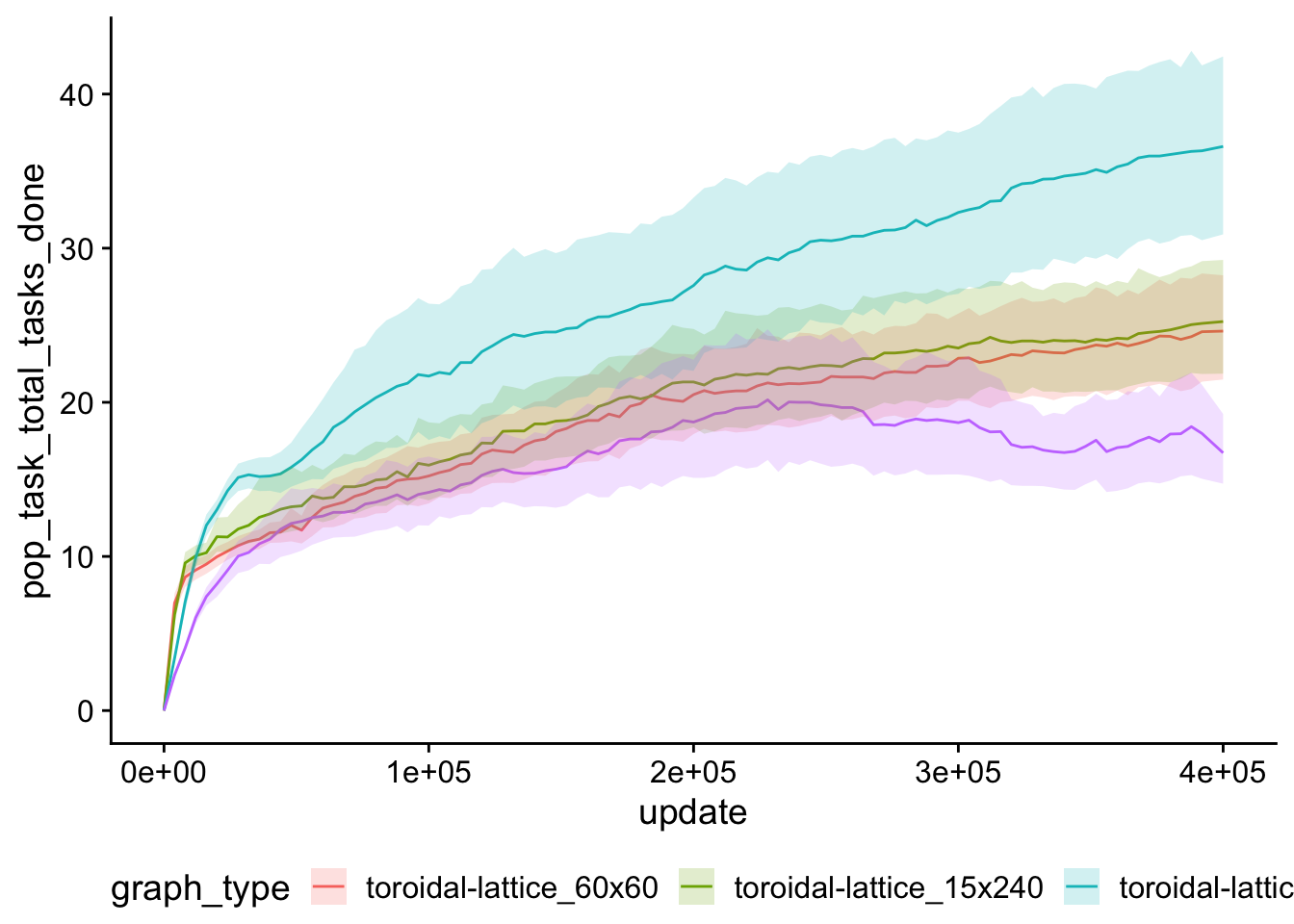
7.9 Average generation over time
time_average_generation_ts <- ggplot(
    data = time_series_data,
    mapping = aes(
      x = update,
      y = time_average_generation,
      color = graph_type,
      fill = graph_type
    )
  ) +
  stat_summary(fun = "mean", geom = "line") +
  stat_summary(
    fun.data = "mean_cl_boot",
    fun.args = list(conf.int = 0.95),
    geom = "ribbon",
    alpha = 0.2,
    linetype = 0
  ) +
  facet_wrap(~ENVIRONMENT_FILE) +
  theme(legend.position = "bottom")

ggsave(
  plot = time_average_generation_ts,
  filename = paste0(
    working_directory,
    "/plots/time_average_generation_ts.pdf"
  ),
  width = 15,
  height = 10
)

time_average_generation_ts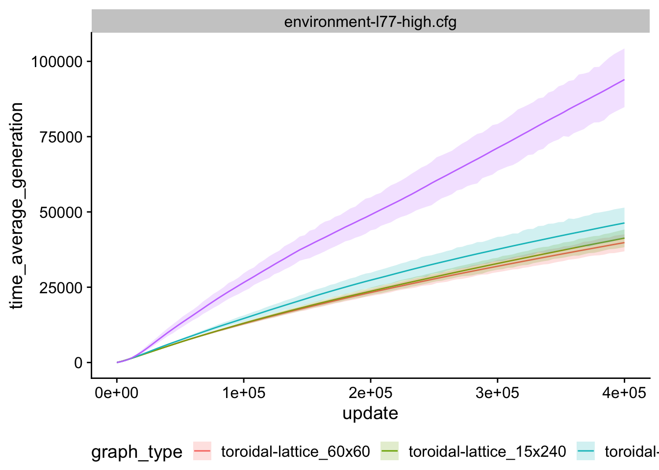
7.10 Graph location info
Analyze graph_birth_info_annotated.csv
# Load summary data from final update
graph_loc_data_path <- paste(
  working_directory,
  "data",
  "graph_birth_info_annotated.csv",
  sep = "/"
)
graph_loc_data <- read_csv(graph_loc_data_path)

graph_loc_data <- graph_loc_data %>%
  mutate(
    graph_type = factor(
      graph_type,
      levels = c(
        "toroidal-lattice_60x60",
        "toroidal-lattice_30x120",
        "toroidal-lattice_15x240",
        "toroidal-lattice_4x900",
        "toroidal-lattice_3x1200",
        "toroidal-lattice_2x1800",
        "cycle"
      )
    ),
    seed = as.factor(seed)
  ) %>%
  filter(
    graph_type %in% focal_graphs
  )
Summarize by seed
graph_loc_data_summary <- graph_loc_data %>%
  group_by(seed, graph_type) %>%
  summarize(
    births_var = var(births),
    births_total = sum(births),
    task_apps_total = sum(task_appearances),
    task_apps_var = var(task_appearances)
  ) %>%
  ungroup()
7.10.1 Total birth Counts
birth_counts_total_plt <- ggplot(
    data = graph_loc_data_summary,
    mapping = aes(
      x = graph_type,
      y = births_total,
      fill = graph_type
    )
  ) +
  geom_flat_violin(
    position = position_nudge(x = .2, y = 0),
    alpha = .8
  ) +
  geom_point(
    mapping=aes(color = graph_type),
    position = position_jitter(width = .15),
    size = .5,
    alpha = 0.8
  ) +
  geom_boxplot(
    width = .1,
    outlier.shape = NA,
    alpha = 0.5
  ) +
  theme(
    legend.position = "none",
    axis.text.x = element_text(
      angle = 30,
      hjust = 1
    )
  )

ggsave(
  filename = paste0(plot_dir, "/birth_counts_total.pdf"),
  plot = birth_counts_total_plt,
  width = 15,
  height = 10
)

birth_counts_total_plt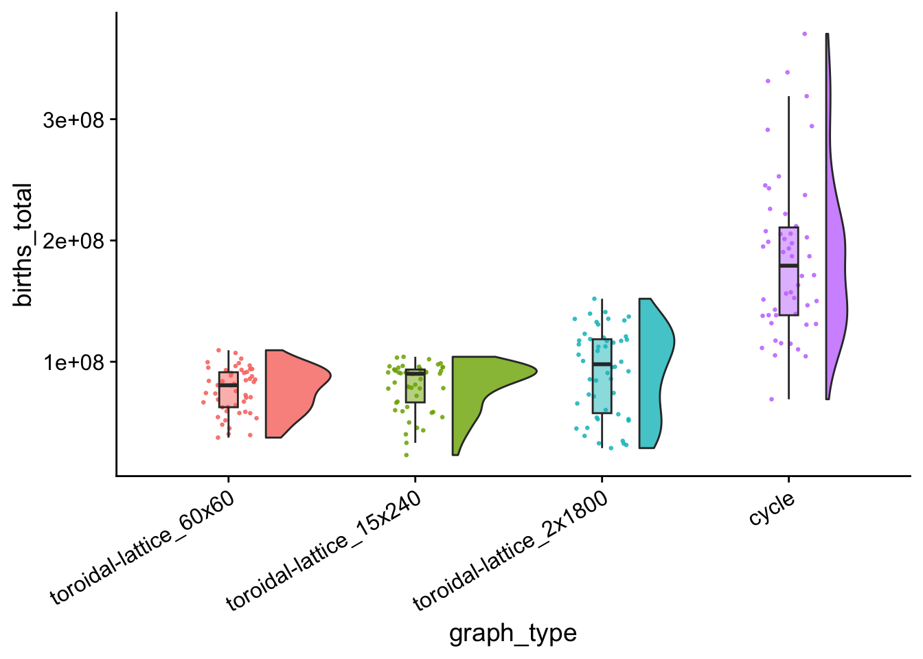
7.10.2 Variance birth Counts
birth_counts_var_plt <- ggplot(
    data = graph_loc_data_summary,
    mapping = aes(
      x = graph_type,
      y = births_var,
      fill = graph_type
    )
  ) +
  geom_flat_violin(
    position = position_nudge(x = .2, y = 0),
    alpha = .8
  ) +
  geom_point(
    mapping=aes(color = graph_type),
    position = position_jitter(width = .15),
    size = .5,
    alpha = 0.8
  ) +
  geom_boxplot(
    width = .1,
    outlier.shape = NA,
    alpha = 0.5
  ) +
  theme(
    legend.position = "none",
    axis.text.x = element_text(
      angle = 30,
      hjust = 1
    )
  )

ggsave(
  filename = paste0(plot_dir, "/birth_counts_var.pdf"),
  plot = birth_counts_var_plt,
  width = 15,
  height = 10
)

birth_counts_var_plt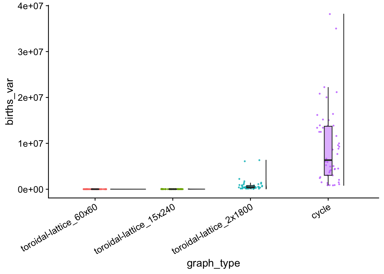
7.10.3 Task appearances total
task_apps_total_plt <- ggplot(
    data = graph_loc_data_summary,
    mapping = aes(
      x = graph_type,
      y = task_apps_total,
      fill = graph_type
    )
  ) +
  geom_flat_violin(
    position = position_nudge(x = .2, y = 0),
    alpha = .8
  ) +
  geom_point(
    mapping=aes(color = graph_type),
    position = position_jitter(width = .15),
    size = .5,
    alpha = 0.8
  ) +
  geom_boxplot(
    width = .1,
    outlier.shape = NA,
    alpha = 0.5
  ) +
  theme(
    legend.position = "none",
    axis.text.x = element_text(
      angle = 30,
      hjust = 1
    )
  )

ggsave(
  filename = paste0(plot_dir, "/task_apps_total.pdf"),
  plot = task_apps_total_plt,
  width = 15,
  height = 10
)

task_apps_total_plt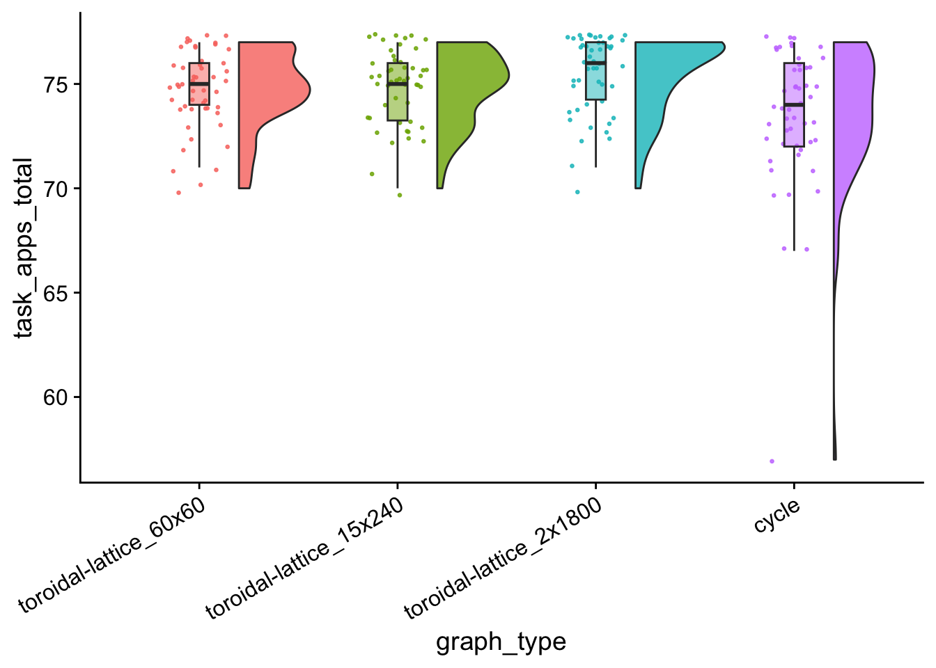
kruskal.test(
  formula = task_apps_total ~ graph_type,
  data = graph_loc_data_summary
)
##
## Kruskal-Wallis rank sum test
##
## data: task_apps_total by graph_type
## Kruskal-Wallis chi-squared = 15.09, df = 3, p-value = 0.001742wc_results <- pairwise.wilcox.test(
x = graph_loc_data_summary$task_apps_total,
g = graph_loc_data_summary$graph_type,
p.adjust.method = "holm",
exact = FALSE
)
wc_results##
## Pairwise comparisons using Wilcoxon rank sum test with continuity correction
##
## data: graph_loc_data_summary$task_apps_total and graph_loc_data_summary$graph_type
##
## toroidal-lattice_60x60 toroidal-lattice_15x240
## toroidal-lattice_15x240 0.771 -
## toroidal-lattice_2x1800 0.125 0.125
## cycle 0.128 0.125
## toroidal-lattice_2x1800
## toroidal-lattice_15x240 -
## toroidal-lattice_2x1800 -
## cycle 0.002
##
## P value adjustment method: holm7.11 Moran’s I results
# Load summary data from final update
morans_i_data_path <- paste(
  working_directory,
  "data",
  "morans_i.csv",
  sep = "/"
)
morans_i_data <- read_csv(morans_i_data_path)

morans_i_data <- morans_i_data %>%
  mutate(
    graph_type = str_split_i(
      graph_file,
      pattern = ".mat",
      1
    )
  ) %>%
  mutate(
    graph_type = factor(
      graph_type,
      levels = c(
        "toroidal-lattice_60x60",
        "toroidal-lattice_30x120",
        "toroidal-lattice_15x240",
        "toroidal-lattice_4x900",
        "toroidal-lattice_3x1200",
        "toroidal-lattice_2x1800",
        "cycle"
      )
    ),
    seed = as.factor(seed)
  ) %>%
  filter(
    graph_type %in% focal_graphs
  )
7.11.1 Clustered task appearances
Summarize statistically significant runs where I > 0.
# Identify number of runs where distribution of task appearances is more
# clustered than we would expect by chance.
clustered_counts <- morans_i_data %>%
  filter(
    (task_morans_i > 0) & (task_p_val <= 0.05)
  ) %>%
  group_by(graph_type) %>%
  summarize(
    n = n()
  )
tasks_clustered_plt <- clustered_counts %>%
ggplot(
aes(
x = graph_type,
y = n,
color = graph_type,
fill = graph_type
)
) +
geom_col() +
theme(
legend.position = "none",
axis.text.x = element_text(
angle = 30,
hjust = 1
)
)
ggsave(
filename = paste0(plot_dir, "/tasks_clustered_plt.pdf"),
plot = tasks_clustered_plt,
width = 15,
height = 10
)
tasks_clustered_plt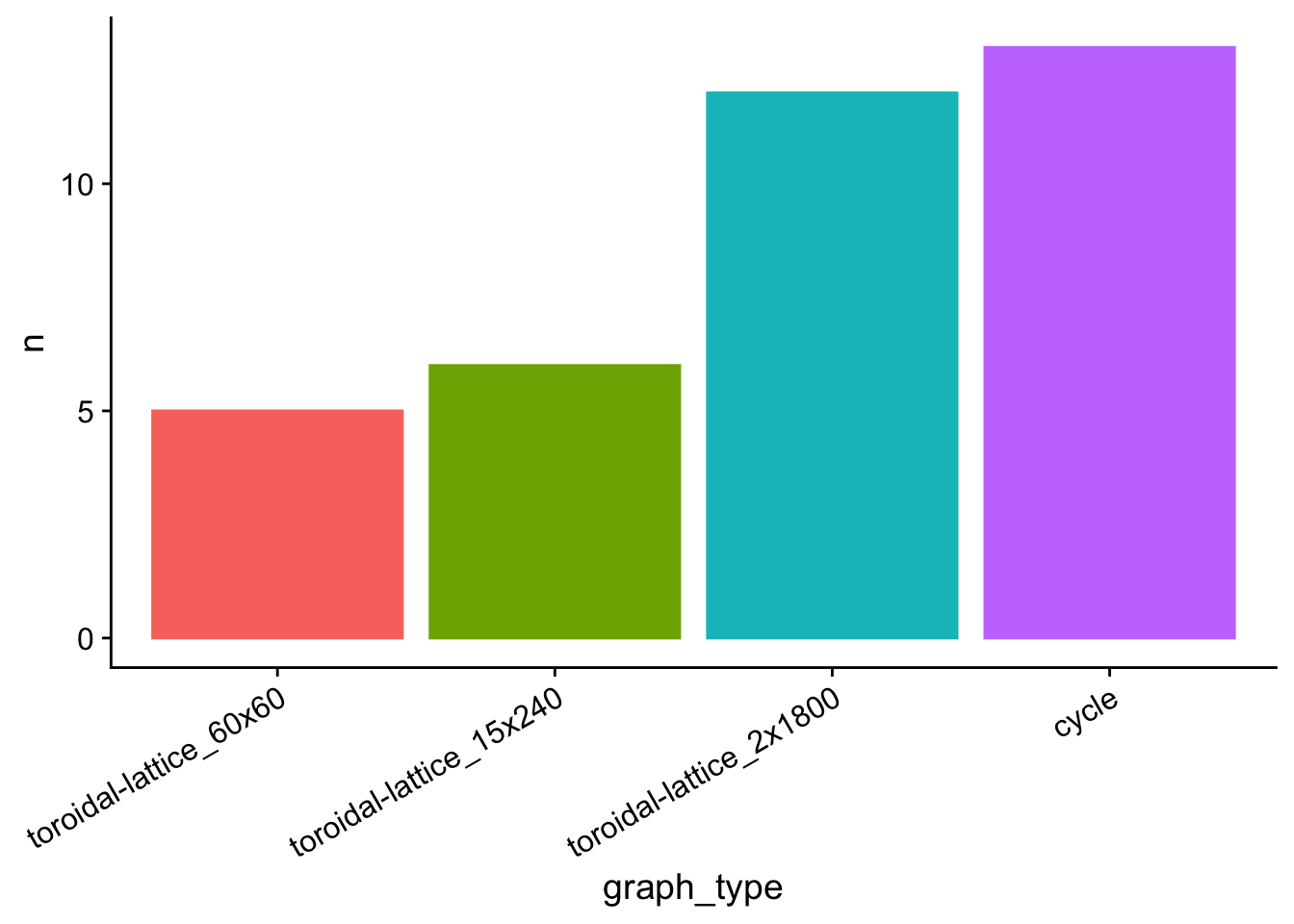
tasks_clustered_i_vals_plt <- morans_i_data %>%
  filter((task_morans_i > 0) & (task_p_val <= 0.05)) %>%
  ggplot(
    mapping = aes(
      x = graph_type,
      y = task_morans_i,
      fill = graph_type
    )
  ) +
  geom_flat_violin(
    position = position_nudge(x = .2, y = 0),
    alpha = .8
  ) +
  geom_point(
    mapping=aes(color = graph_type),
    position = position_jitter(width = .15),
    size = .5,
    alpha = 0.8
  ) +
  geom_boxplot(
    width = .1,
    outlier.shape = NA,
    alpha = 0.5
  ) +
  theme(
    legend.position = "none",
    axis.text.x = element_text(
      angle = 30,
      hjust = 1
    )
  )

ggsave(
  filename = paste0(plot_dir, "/tasks_clustered_i_vals_plt.pdf"),
  plot = tasks_clustered_i_vals_plt,
  width = 15,
  height = 10
)

tasks_clustered_i_vals_plt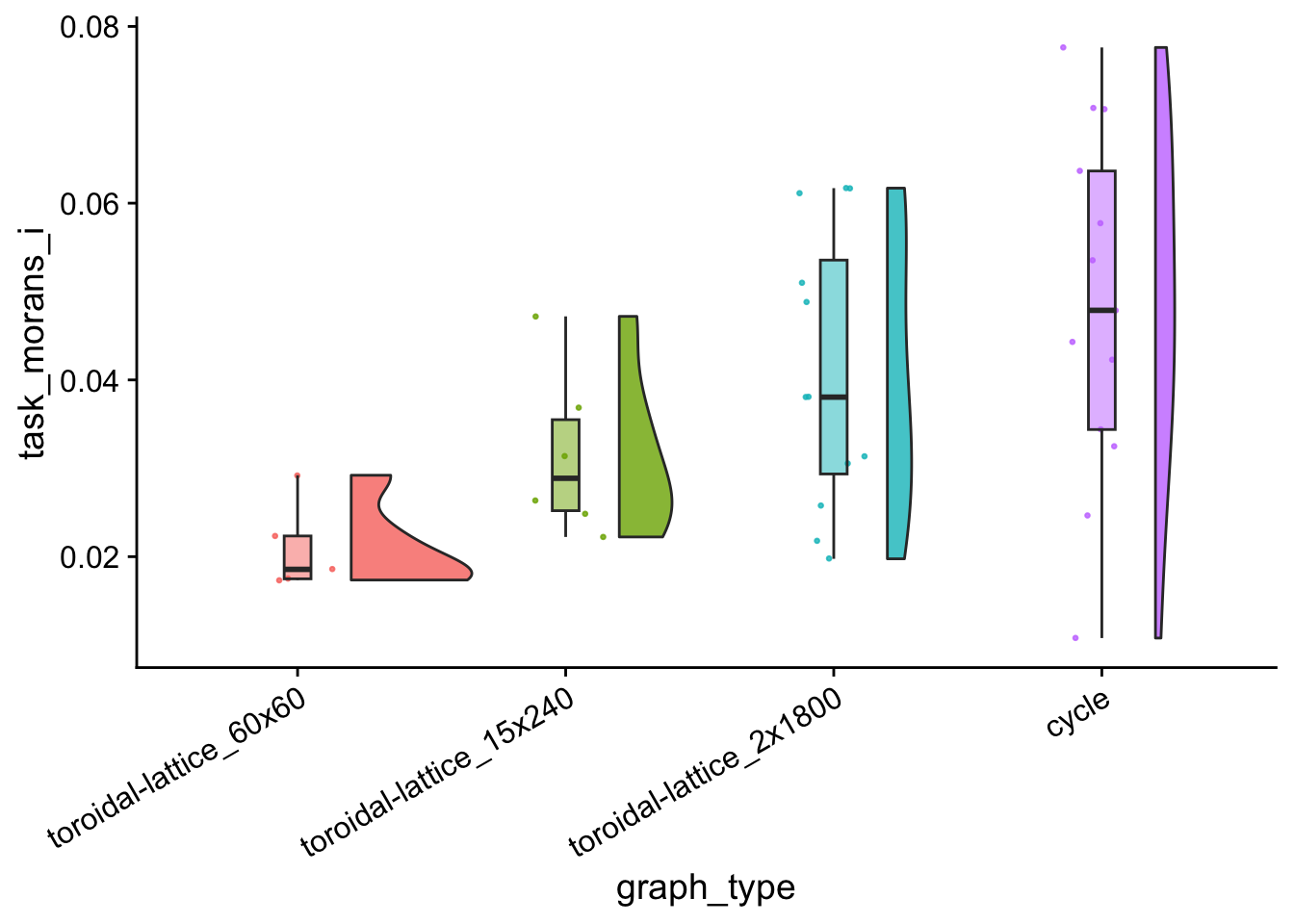
7.11.2 Clustered birth counts
births_clustered_plot <- morans_i_data %>%
  filter((birth_morans_i > 0) & (birth_p_val <= 0.05)) %>%
  ggplot(
    aes(
      x = graph_type,
      color = graph_type,
      fill = graph_type
    )
  ) +
  geom_bar() +
  theme(
    legend.position = "none",
    axis.text.x = element_text(
      angle = 30,
      hjust = 1
    )
  )

ggsave(
  filename = paste0(plot_dir, "/births_clustered_plot.pdf"),
  plot = births_clustered_plot,
  width = 15,
  height = 10
)

births_clustered_plot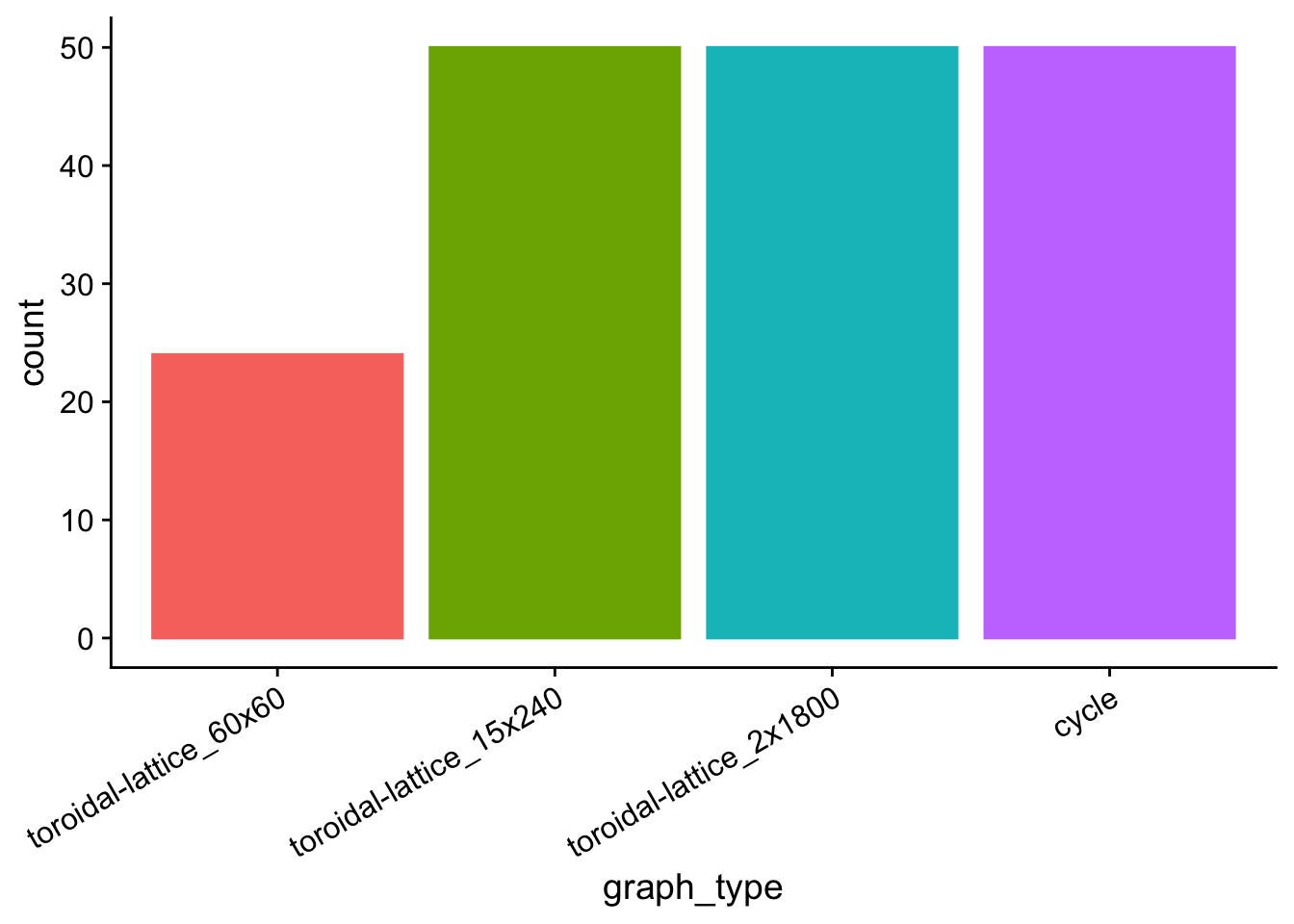
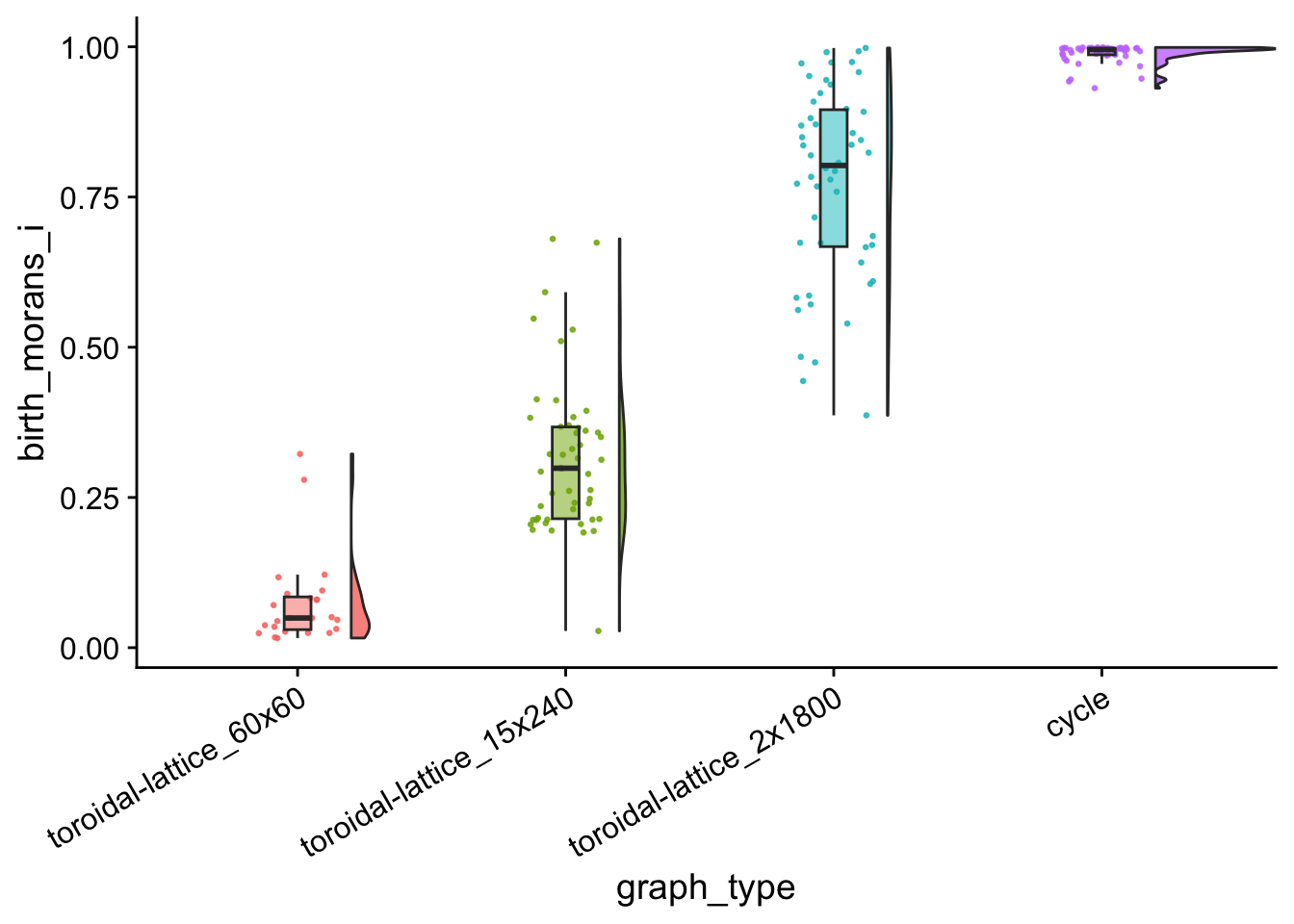
birth_clustered_i_vals_plt <- morans_i_data %>%
  filter((birth_morans_i > 0) & (birth_p_val <= 0.05)) %>%
  ggplot(
    mapping = aes(
      x = graph_type,
      y = birth_morans_i,
      fill = graph_type
    )
  ) +
  geom_flat_violin(
    position = position_nudge(x = .2, y = 0),
    alpha = .8
  ) +
  geom_point(
    mapping=aes(color = graph_type),
    position = position_jitter(width = .15),
    size = .5,
    alpha = 0.8
  ) +
  geom_boxplot(
    width = .1,
    outlier.shape = NA,
    alpha = 0.5
  ) +
  theme(
    legend.position = "none",
    axis.text.x = element_text(
      angle = 30,
      hjust = 1
    )
  )

ggsave(
  filename = paste0(plot_dir, "/birth_clustered_i_vals_plt.pdf"),
  plot = birth_clustered_i_vals_plt,
  width = 15,
  height = 10
)

birth_clustered_i_vals_plt