Chapter 5 Simple model - Squished toroid experiment analyses

5.1 Setup and Dependencies

library(tidyverse)
library(cowplot)
library(RColorBrewer)
library(khroma)
library(rstatix)
library(knitr)
library(kableExtra)
library(infer)
source("https://gist.githubusercontent.com/benmarwick/2a1bb0133ff568cbe28d/raw/fb53bd97121f7f9ce947837ef1a4c65a73bffb3f/geom_flat_violin.R")

# Check if Rmd is being compiled using bookdown
bookdown <- exists("bookdown_build")

experiment_slug <- "lattice-experiments"
working_directory <- paste(
  "experiments",
  "mabe2-exps",
  experiment_slug,
  sep = "/"
)
# Adjust working directory if being knitted for bookdown build.
if (bookdown) {
  working_directory <- paste0(
    bookdown_wd_prefix,
    working_directory
  )
}

# Configure our default graphing theme
theme_set(theme_cowplot())
# Create a directory to store plots
plot_dir <- paste(
  working_directory,
  "rmd_plots",
  sep = "/"
)

dir.create(
  plot_dir,
  showWarnings = FALSE
)

5.2 Max organism data analyses

max_generation <- 100000
max_org_data_path <- paste(
  working_directory,
  "data",
  "combined_max_org_data.csv",
  sep = "/"
)
# Data file has time series
max_org_data_ts <- read_csv(max_org_data_path)
max_org_data_ts <- max_org_data_ts %>%
  mutate(
    landscape = as.factor(landscape),
    structure = factor(
      structure,
      levels = c(
        "1_3600",
        "2_1800",
        "3_1200",
        "4_900",
        "15_240",
        "30_120",
        "60_60"
      )
    ),
  ) %>%
  mutate(
    valleys_crossed = case_when(
      landscape == "Valley crossing" ~ round(log(fitness, base = 1.5)),
      .default = 0
    )
  )
# Get tibble with just final generation
max_org_data <- max_org_data_ts %>%
  filter(generation == max_generation)

Check that replicate count for each condition matches expectations.

run_summary <- max_org_data %>%
  group_by(landscape, structure) %>%
  summarize(
    n = n()
  )
print(run_summary, n = 30)

## # A tibble: 21 × 3
## # Groups:   landscape [3]
##    landscape       structure     n
##    <fct>           <fct>     <int>
##  1 Multipath       1_3600       50
##  2 Multipath       2_1800       50
##  3 Multipath       3_1200       50
##  4 Multipath       4_900        50
##  5 Multipath       15_240       50
##  6 Multipath       30_120       50
##  7 Multipath       60_60        50
##  8 Single gradient 1_3600       50
##  9 Single gradient 2_1800       50
## 10 Single gradient 3_1200       50
## 11 Single gradient 4_900        50
## 12 Single gradient 15_240       50
## 13 Single gradient 30_120       50
## 14 Single gradient 60_60        50
## 15 Valley crossing 1_3600       50
## 16 Valley crossing 2_1800       50
## 17 Valley crossing 3_1200       50
## 18 Valley crossing 4_900        50
## 19 Valley crossing 15_240       50
## 20 Valley crossing 30_120       50
## 21 Valley crossing 60_60        50

5.2.1 Fitness in smooth gradient landscape

single_gradient_final_fitness_plt <- ggplot(
    data = filter(max_org_data, landscape == "Single gradient"),
    mapping = aes(
      x = structure,
      y = fitness,
      fill = structure
    )
  ) +
  geom_flat_violin(
    position = position_nudge(x = .2, y = 0),
    alpha = .8
  ) +
  geom_point(
    mapping = aes(color = structure),
    position = position_jitter(width = .15),
    size = .5,
    alpha = 0.8
  ) +
  geom_boxplot(
    width = .1,
    outlier.shape = NA,
    alpha = 0.5
  ) +
  theme(
    legend.position = "none",
    axis.text.x = element_text(
      angle = 30,
      hjust = 1
    )
  )

ggsave(
  filename = paste0(plot_dir, "/single_gradient_final_fitness.pdf"),
  plot = single_gradient_final_fitness_plt,
  width = 15,
  height = 10
)

single_gradient_final_fitness_plt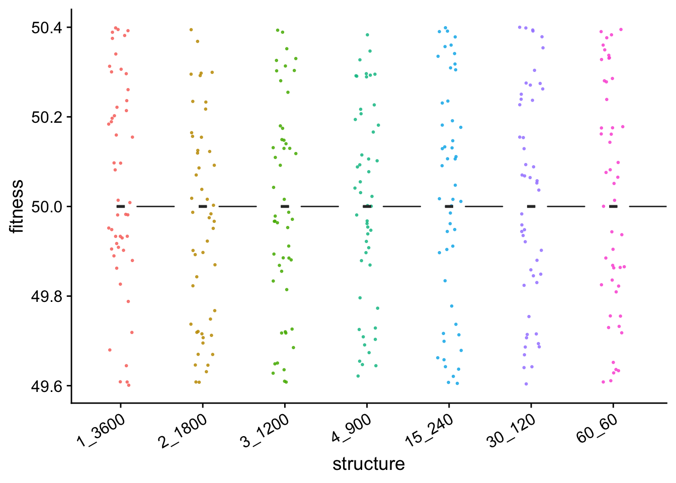

Max fitness over time

single_gradient_fitness_ts_plt <- ggplot(
    data = filter(max_org_data_ts, landscape == "Single gradient"),
    mapping = aes(
      x = generation,
      y = fitness,
      color = structure,
      fill = structure
    )
  ) +
  stat_summary(fun = "mean", geom = "line") +
  stat_summary(
    fun.data = "mean_cl_boot",
    fun.args = list(conf.int = 0.95),
    geom = "ribbon",
    alpha = 0.2,
    linetype = 0
  ) +
  theme(legend.position = "bottom")

ggsave(
  plot = single_gradient_fitness_ts_plt,
  filename = paste0(
    plot_dir,
    "/single_gradient_fitness_ts.pdf"
  ),
  width = 15,
  height = 10
)

single_gradient_fitness_ts_plt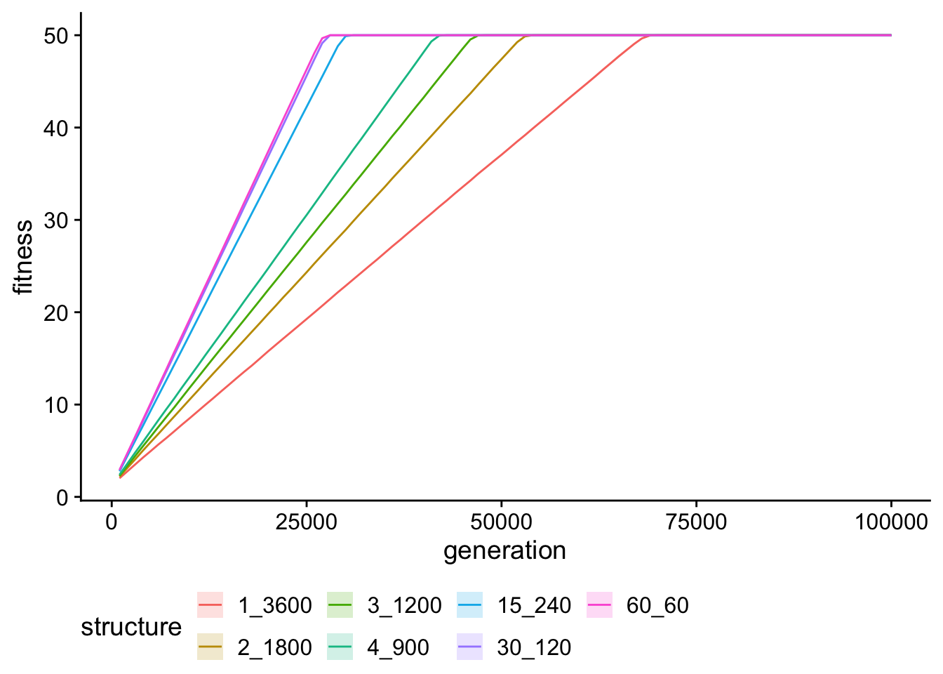

Time to maximum fitness

# Find all rows with maximum fitness value, then get row with minimum generation,
#  then project out expected generation to max (for runs that didn't finish)
max_possible_fit = 50
time_to_max_single_gradient <- max_org_data_ts %>%
  filter(landscape == "Single gradient") %>%
  group_by(rep, structure) %>%
  slice_max(
    fitness,
    n = 1
  ) %>%
  slice_min(
    generation,
    n = 1
  ) %>%
  mutate(
    proj_gen_max = (max_possible_fit / fitness) * generation
  )

single_gradient_gen_max_proj_plt <- ggplot(
    data = time_to_max_single_gradient,
    mapping = aes(
      x = structure,
      y = proj_gen_max,
      fill = structure
    )
  ) +
  geom_flat_violin(
    position = position_nudge(x = .2, y = 0),
    alpha = .8
  ) +
  geom_point(
    mapping = aes(color = structure),
    position = position_jitter(width = .15),
    size = .5,
    alpha = 0.8
  ) +
  geom_boxplot(
    width = .1,
    outlier.shape = NA,
    alpha = 0.5
  ) +
  scale_y_log10(
    guide = "axis_logticks"
  ) +
  # scale_y_continuous(
  #   trans="pseudo_log",
  #   breaks = c(10, 100, 1000, 10000, 100000, 1000000)
  #   ,limits = c(10, 100, 1000, 10000, 100000, 1000000)
  # ) +
  geom_hline(
    yintercept = max_generation,
    linetype = "dashed"
  ) +
  theme(
    legend.position = "none",
    axis.text.x = element_text(
      angle = 30,
      hjust = 1
    )
  )

ggsave(
  filename = paste0(plot_dir, "/single_gradient_gen_max_proj.pdf"),
  plot = single_gradient_gen_max_proj_plt,
  width = 15,
  height = 10
)

single_gradient_gen_max_proj_plt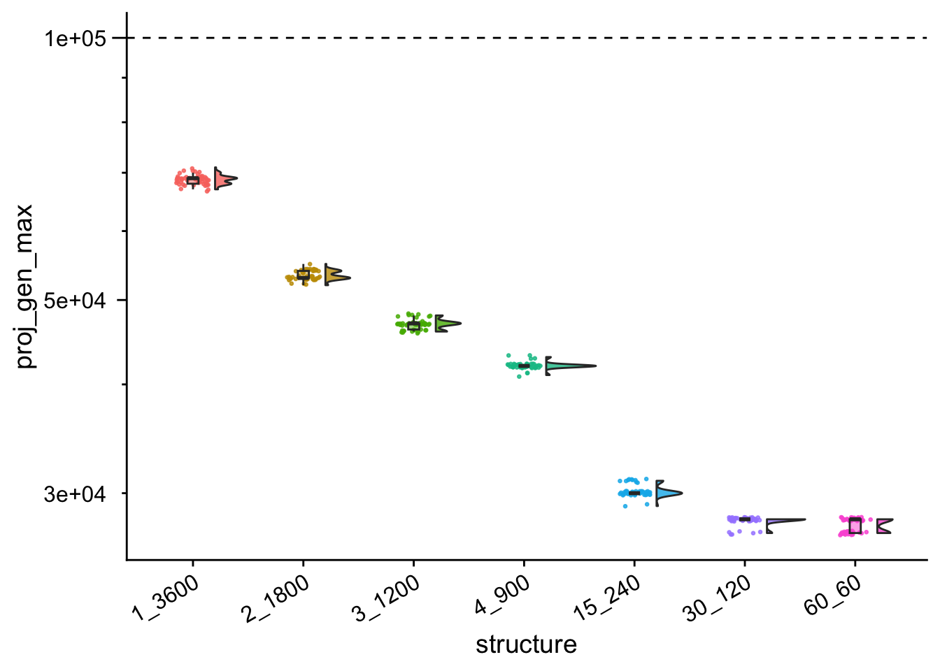

Rank ordering of time to max fitness values

time_to_max_single_gradient %>%
  group_by(structure) %>%
  summarize(
    reps = n(),
    median_proj_gen = median(proj_gen_max),
    mean_proj_gen = mean(proj_gen_max)
  ) %>%
  arrange(
    mean_proj_gen
  )

## # A tibble: 7 × 4
##   structure  reps median_proj_gen mean_proj_gen
##   <fct>     <int>           <dbl>         <dbl>
## 1 60_60        50           28000         27540
## 2 30_120       50           28000         27880
## 3 15_240       50           30000         30160
## 4 4_900        50           42000         42020
## 5 3_1200       50           47000         46900
## 6 2_1800       50           53000         53340
## 7 1_3600       50           69000         68700

kruskal.test(
  formula = proj_gen_max ~ structure,
  data = time_to_max_single_gradient
)

## 
##  Kruskal-Wallis rank sum test
## 
## data:  proj_gen_max by structure
## Kruskal-Wallis chi-squared = 341.17, df = 6, p-value < 2.2e-16

wc_results <- pairwise.wilcox.test(
  x = time_to_max_single_gradient$proj_gen_max,
  g = time_to_max_single_gradient$structure,
  p.adjust.method   = "holm",
  exact = FALSE
)

single_gradient_proj_gen_max_wc_table <- kbl(wc_results$p.value) %>%
  kable_styling()

save_kable(
  single_gradient_proj_gen_max_wc_table,
  paste0(plot_dir, "/single_gradient_proj_gen_max_wc_table.pdf")
)
single_gradient_proj_gen_max_wc_table

	1_3600	2_1800	3_1200	4_900	15_240	30_120
2_1800	0	NA	NA	NA	NA	NA
3_1200	0	0	NA	NA	NA	NA
4_900	0	0	0	NA	NA	NA
15_240	0	0	0	0	NA	NA
30_120	0	0	0	0	0	NA
60_60	0	0	0	0	0	0.0001966

library(boot)
# Define sample mean function
samplemean <- function(x, d) {
  return(mean(x[d]))
}

summary_gen_to_max <- tibble(
  structure = character(),
  proj_gen_max_mean = double(),
  proj_gen_max_mean_ci_low = double(),
  proj_gen_max_mean_ci_high = double()
)

structures <- levels(time_to_max_single_gradient$structure)
for (struct in structures) {
  boot_result <- boot(
    data = filter(
      time_to_max_single_gradient,
      structure == struct
    )$proj_gen_max,
    statistic = samplemean,
    R = 10000
  )
  result_ci <- boot.ci(boot_result, conf = 0.99, type = "perc")
  m <- result_ci$t0
  low <- result_ci$percent[4]
  high <- result_ci$percent[5]

  summary_gen_to_max <- summary_gen_to_max %>%
    add_row(
      structure = struct,
      proj_gen_max_mean = m,
      proj_gen_max_mean_ci_low = low,
      proj_gen_max_mean_ci_high = high
    )
}

wm_median <- median(
  filter(time_to_max_single_gradient, structure == "well_mixed")$proj_gen_max
)

simple_time_to_max_plt <- ggplot(
    data = summary_gen_to_max,
    mapping = aes(
      x = structure,
      y = proj_gen_max_mean,
      fill = structure,
      color = structure
    )
  ) +
  # geom_point() +
  geom_col() +
  geom_linerange(
    aes(
      ymin = proj_gen_max_mean_ci_low,
      ymax = proj_gen_max_mean_ci_high
    ),
    color = "black",
    linewidth = 0.75,
    lineend = "round"
  ) +
  # scale_y_log10(
  #   guide = "axis_logticks"
  # ) +
  geom_hline(
    yintercept = max_generation,
    linetype = "dashed"
  ) +
  geom_hline(
    yintercept = wm_median,
    linetype = "dotted",
    color = "orange"
  ) +
  scale_color_discreterainbow() +
  scale_fill_discreterainbow() +
  coord_flip() +
  theme(
    legend.position = "none",
    axis.text.x = element_text(
      angle = 30,
      hjust = 1
    )
  )

ggsave(
  filename = paste0(plot_dir, "/simple_time_to_max.pdf"),
  plot = simple_time_to_max_plt,
  width = 8,
  height = 4
)

simple_time_to_max_plt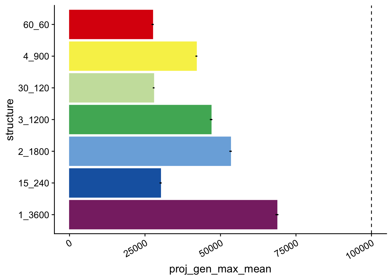

5.2.2 Fitness in multi-path landscape

multipath_final_fitness_plt <- ggplot(
    data = filter(max_org_data, landscape == "Multipath"),
    mapping = aes(
      x = structure,
      y = fitness,
      fill = structure
    )
  ) +
  # geom_flat_violin(
  #   position = position_nudge(x = .2, y = 0),
  #   alpha = .8
  # ) +
  geom_point(
    mapping = aes(color = structure),
    position = position_jitter(width = .15),
    size = .5,
    alpha = 0.8
  ) +
  geom_boxplot(
    width = .3,
    outlier.shape = NA,
    alpha = 0.5
  ) +
  scale_color_discreterainbow() +
  scale_fill_discreterainbow() +
  theme(
    legend.position = "none",
    axis.text.x = element_text(
      angle = 30,
      hjust = 1
    )
  )

ggsave(
  filename = paste0(plot_dir, "/multipath_final_fitness.pdf"),
  plot = multipath_final_fitness_plt,
  width = 6,
  height = 4
)

multipath_final_fitness_plt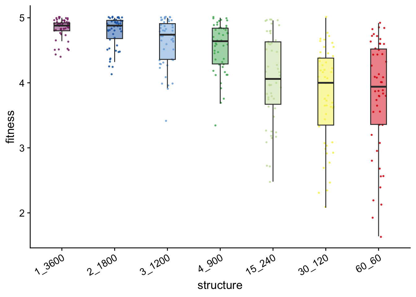

Max fitness over time

multipath_fitness_ts_plt <- ggplot(
    data = filter(max_org_data_ts, landscape == "Multipath"),
    mapping = aes(
      x = generation,
      y = fitness,
      color = structure,
      fill = structure
    )
  ) +
  stat_summary(fun = "mean", geom = "line") +
  stat_summary(
    fun.data = "mean_cl_boot",
    fun.args = list(conf.int = 0.95),
    geom = "ribbon",
    alpha = 0.2,
    linetype = 0
  ) +
  theme(legend.position = "bottom")

ggsave(
  plot = multipath_fitness_ts_plt,
  filename = paste0(
    plot_dir,
    "/multipath_fitness_ts.pdf"
  ),
  width = 15,
  height = 10
)

multipath_fitness_ts_plt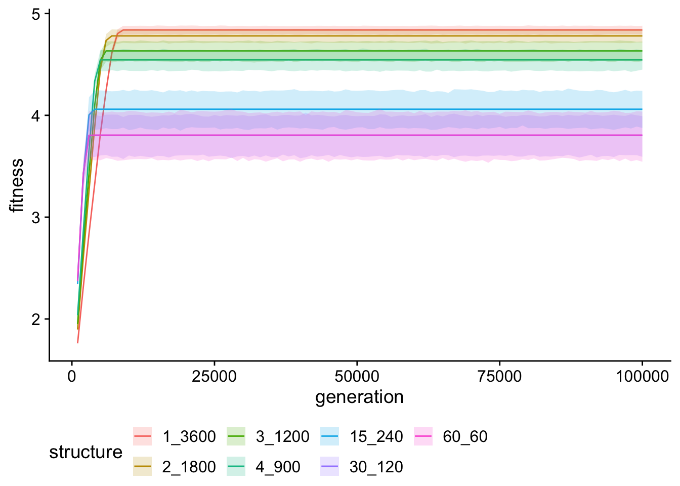

Rank ordering of fitness values

max_org_data %>%
  filter(landscape == "Multipath") %>%
  group_by(structure) %>%
  summarize(
    reps = n(),
    median_fitness = median(fitness),
    mean_fitness = mean(fitness)
  ) %>%
  arrange(
    desc(mean_fitness)
  )

## # A tibble: 7 × 4
##   structure  reps median_fitness mean_fitness
##   <fct>     <int>          <dbl>        <dbl>
## 1 1_3600       50           4.88         4.84
## 2 2_1800       50           4.88         4.78
## 3 3_1200       50           4.74         4.63
## 4 4_900        50           4.64         4.54
## 5 15_240       50           4.06         4.06
## 6 60_60        50           3.94         3.81
## 7 30_120       50           4            3.80

kruskal.test(
  formula = fitness ~ structure,
  data = filter(max_org_data, landscape == "Multipath")
)

## 
##  Kruskal-Wallis rank sum test
## 
## data:  fitness by structure
## Kruskal-Wallis chi-squared = 144.73, df = 6, p-value < 2.2e-16

wc_results <- pairwise.wilcox.test(
  x = filter(max_org_data, landscape == "Multipath")$fitness,
  g = filter(max_org_data, landscape == "Multipath")$structure,
  p.adjust.method   = "holm",
  exact = FALSE
)

mp_fitness_wc_table <- kbl(wc_results$p.value) %>%
  kable_styling()

save_kable(
  mp_fitness_wc_table,
  paste0(plot_dir, "/multipath_fitness_wc_table.pdf")
)
mp_fitness_wc_table

	1_3600	2_1800	3_1200	4_900	15_240	30_120
2_1800	1.0000000	NA	NA	NA	NA	NA
3_1200	0.0389539	0.2309342	NA	NA	NA	NA
4_900	0.0000552	0.0022081	0.6036094	NA	NA	NA
15_240	0.0000000	0.0000001	0.0000387	0.0022081	NA	NA
30_120	0.0000000	0.0000000	0.0000000	0.0000003	0.4456978	NA
60_60	0.0000000	0.0000000	0.0000002	0.0000094	0.6036094	1

5.2.3 Valleys crossed in valley-crossing landscape

valleycrossing_valleys_plt <- ggplot(
    data = filter(max_org_data, landscape == "Valley crossing"),
    mapping = aes(
      x = structure,
      y = valleys_crossed,
      fill = structure
    )
  ) +
  # geom_flat_violin(
  #   position = position_nudge(x = .2, y = 0),
  #   alpha = .8
  # ) +
  geom_point(
    mapping = aes(color = structure),
    position = position_jitter(width = .15),
    size = .5,
    alpha = 0.8
  ) +
  geom_boxplot(
    width = .3,
    outlier.shape = NA,
    alpha = 0.5
  ) +
  scale_color_discreterainbow() +
  scale_fill_discreterainbow() +
  theme(
    legend.position = "none",
    axis.text.x = element_text(
      angle = 30,
      hjust = 1
    )
  )
ggsave(
  filename = paste0(plot_dir, "/valleycrossing_valleys_crossed.pdf"),
  plot = valleycrossing_valleys_plt,
  width = 6,
  height = 4
)

valleycrossing_valleys_plt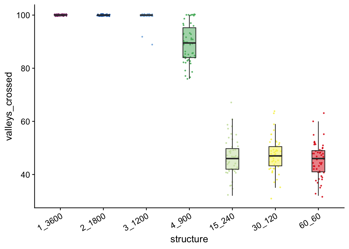

vc <- max_org_data %>%
  filter(landscape == "Valley crossing") %>%
  group_by(structure) %>%
  summarize(
    reps = n(),
    median_valleys_crossed = median(valleys_crossed),
    mean_valleys_crossed = mean(valleys_crossed),
    min_valleys_crossed = min(valleys_crossed)
  ) %>%
  arrange(
    desc(mean_valleys_crossed)
  )
vc

## # A tibble: 7 × 5
##   structure  reps median_valleys_crossed mean_valleys_crossed
##   <fct>     <int>                  <dbl>                <dbl>
## 1 1_3600       50                  100                  100  
## 2 2_1800       50                  100                  100  
## 3 3_1200       50                  100                   99.6
## 4 4_900        50                   89.5                 89.3
## 5 30_120       50                   47                   47.2
## 6 15_240       50                   46                   46.6
## 7 60_60        50                   46                   45.5
## # ℹ 1 more variable: min_valleys_crossed <dbl>

vc$min_valleys_crossed

## [1] 100 100  89  76  31  32  32

kruskal.test(
  formula = valleys_crossed ~ structure,
  data = filter(max_org_data, landscape == "Valley crossing")
)

## 
##  Kruskal-Wallis rank sum test
## 
## data:  valleys_crossed by structure
## Kruskal-Wallis chi-squared = 309.49, df = 6, p-value < 2.2e-16

wc_results <- pairwise.wilcox.test(
  x = filter(max_org_data, landscape == "Valley crossing")$valleys_crossed,
  g = filter(max_org_data, landscape == "Valley crossing")$structure,
  p.adjust.method   = "holm",
  exact = FALSE
)

vc_valleys_crossed_wc_table <- kbl(wc_results$p.value) %>%
  kable_styling()

save_kable(
  vc_valleys_crossed_wc_table,
  paste0(plot_dir, "/valley_crossing_valleys_wc_table.pdf")
)
vc_valleys_crossed_wc_table

	1_3600	2_1800	3_1200	4_900	15_240	30_120
2_1800	NaN	NA	NA	NA	NA	NA
3_1200	0.796952	0.796952	NA	NA	NA	NA
4_900	0.000000	0.000000	0	NA	NA	NA
15_240	0.000000	0.000000	0	0	NA	NA
30_120	0.000000	0.000000	0	0	0.9787605	NA
60_60	0.000000	0.000000	0	0	0.9787605	0.796952