Chapter 6 Avida - Varied graph structure experiment analyses
6.1 Dependencies and setup
library(tidyverse)
library(cowplot)
library(RColorBrewer)
library(khroma)
library(rstatix)
library(knitr)
library(kableExtra)
source("https://gist.githubusercontent.com/benmarwick/2a1bb0133ff568cbe28d/raw/fb53bd97121f7f9ce947837ef1a4c65a73bffb3f/geom_flat_violin.R")
# Check if Rmd is being compiled using bookdown
bookdown <- exists("bookdown_build")experiment_slug <- "2025-04-17-vary-structs"
working_directory <- paste(
"experiments",
experiment_slug,
"analysis",
sep = "/"
)
# Adjust working directory if being knitted for bookdown build.
if (bookdown) {
working_directory <- paste0(
bookdown_wd_prefix,
working_directory
)
}# Configure our default graphing theme
theme_set(theme_cowplot())
# Create a directory to store plots
plot_dir <- paste(
working_directory,
"plots",
sep = "/"
)
dir.create(
plot_dir,
showWarnings = FALSE
)focal_graphs <- c(
"star",
"random-waxman",
"comet-kite",
"linear-chain",
"cycle",
"clique-ring",
"toroidal-lattice",
"well-mixed",
"wheel",
"windmill"
)
# Load summary data from final update
data_path <- paste(
working_directory,
"data",
"summary.csv",
sep = "/"
)
data <- read_csv(data_path)
data <- data %>%
mutate(
graph_type = factor(
graph_type,
levels = c(
"star",
"random-waxman",
"comet-kite",
"linear-chain",
"cycle",
"clique-ring",
"toroidal-lattice",
"well-mixed",
"wheel",
"windmill"
)
),
ENVIRONMENT_FILE = as.factor(ENVIRONMENT_FILE)
)
data <- data %>% filter(
graph_type %in% focal_graphs
)
data <- data %>% filter(reached_target_update)time_series_path <- paste(
working_directory,
"data",
"time_series.csv",
sep = "/"
)
time_series_data <- read_csv(time_series_path)
time_series_data <- time_series_data %>%
mutate(
graph_type = factor(
graph_type,
levels = c(
"star",
"random-waxman",
"comet-kite",
"linear-chain",
"cycle",
"clique-ring",
"toroidal-lattice",
"well-mixed",
"wheel",
"windmill"
)
),
ENVIRONMENT_FILE = as.factor(ENVIRONMENT_FILE),
seed = as.factor(seed)
)
time_series_data <- time_series_data %>% filter(seed %in% data$seed)
time_series_data <- time_series_data %>% filter(
graph_type %in% focal_graphs
)# Check that all runs completed
data %>%
filter(update == 400000) %>%
group_by(graph_type) %>%
summarize(
n = n()
)## # A tibble: 10 × 2
## graph_type n
## <fct> <int>
## 1 star 50
## 2 random-waxman 50
## 3 comet-kite 50
## 4 linear-chain 50
## 5 cycle 50
## 6 clique-ring 50
## 7 toroidal-lattice 50
## 8 well-mixed 50
## 9 wheel 50
## 10 windmill 506.2 Number of tasks completed
pop_tasks_total_plt <- ggplot(
  data = data,
  mapping = aes(
    x = graph_type,
    y = pop_task_total,
    fill = graph_type
  )
) +
  geom_flat_violin(
    position = position_nudge(x = .2, y = 0),
    alpha = .8
  ) +
  geom_point(
    mapping=aes(color = graph_type),
    position = position_jitter(width = .15),
    size = .5,
    alpha = 0.8
  ) +
  geom_boxplot(
    width = .1,
    outlier.shape = NA,
    alpha = 0.5
  ) +
  theme(
    legend.position = "none",
    axis.text.x = element_text(
      angle = 30,
      hjust = 1
    )
  )

ggsave(
  filename = paste0(plot_dir, "/pop_tasks_total.pdf"),
  plot = pop_tasks_total_plt,
  width = 15,
  height = 10
)

pop_tasks_total_plt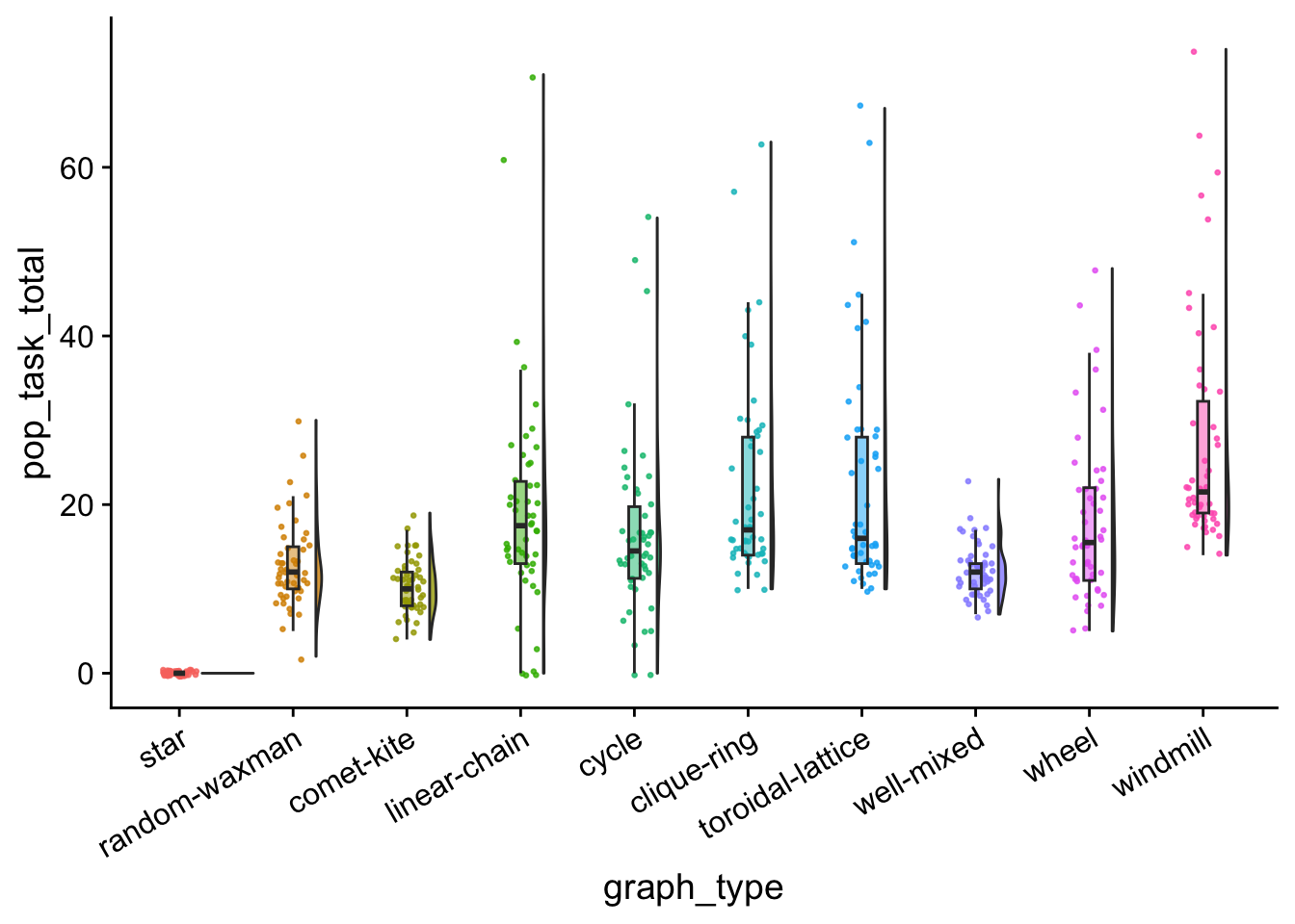
data %>%
  group_by(graph_type) %>%
  summarize(
    reps = n(),
    median_pop_tasks = median(pop_task_total),
    mean_pop_tasks = mean(pop_task_total)
  ) %>%
  arrange(
    desc(mean_pop_tasks)
  )
## # A tibble: 10 × 4
## graph_type reps median_pop_tasks mean_pop_tasks
## <fct> <int> <dbl> <dbl>
## 1 windmill 50 21.5 27.4
## 2 toroidal-lattice 50 16 22.4
## 3 clique-ring 50 17 22.1
## 4 linear-chain 50 17.5 19.1
## 5 wheel 50 15.5 17.8
## 6 cycle 50 14.5 16.6
## 7 random-waxman 50 12 12.8
## 8 well-mixed 50 12 12.2
## 9 comet-kite 50 10 10.3
## 10 star 50 0 0kruskal.test(
formula = pop_task_total ~ graph_type,
data = data
)##
## Kruskal-Wallis rank sum test
##
## data: pop_task_total by graph_type
## Kruskal-Wallis chi-squared = 252.46, df = 9, p-value < 2.2e-16wc_results <- pairwise.wilcox.test(
x = data$pop_task_total,
g = data$graph_type,
p.adjust.method = "holm",
exact = FALSE
)
pop_task_wc_table <- kbl(wc_results$p.value) %>% kable_styling()
save_kable(pop_task_wc_table, paste0(plot_dir, "/pop_task_wc_table.pdf"))
pop_task_wc_table| star | random-waxman | comet-kite | linear-chain | cycle | clique-ring | toroidal-lattice | well-mixed | wheel | |
|---|---|---|---|---|---|---|---|---|---|
| random-waxman | 0 | NA | NA | NA | NA | NA | NA | NA | NA |
| comet-kite | 0 | 0.0755715 | NA | NA | NA | NA | NA | NA | NA |
| linear-chain | 0 | 0.0040473 | 0.0000027 | NA | NA | NA | NA | NA | NA |
| cycle | 0 | 0.1530200 | 0.0002750 | 1.0000000 | NA | NA | NA | NA | NA |
| clique-ring | 0 | 0.0000008 | 0.0000000 | 1.0000000 | 0.0702670 | NA | NA | NA | NA |
| toroidal-lattice | 0 | 0.0000297 | 0.0000000 | 1.0000000 | 0.3032752 | 1.0000000 | NA | NA | NA |
| well-mixed | 0 | 1.0000000 | 0.0542973 | 0.0002739 | 0.0505844 | 0.0000000 | 0.0000018 | NA | NA |
| wheel | 0 | 0.0681554 | 0.0000297 | 1.0000000 | 1.0000000 | 0.2644489 | 0.6033308 | 0.0280284 | NA |
| windmill | 0 | 0.0000000 | 0.0000000 | 0.0058779 | 0.0000035 | 0.0302955 | 0.0302955 | 0.0000000 | 0.000275 |
6.3 Dominant tasks
dom_tasks_total_plt <- ggplot(
  data = data,
  mapping = aes(
    x = graph_type,
    y = dom_task_total,
    fill = graph_type
  )
) +
  geom_flat_violin(
    position = position_nudge(x = .2, y = 0),
    alpha = .8
  ) +
  geom_point(
    mapping=aes(color = graph_type),
    position = position_jitter(width = .15),
    size = .5,
    alpha = 0.8
  ) +
  geom_boxplot(
    width = .1,
    outlier.shape = NA,
    alpha = 0.5
  ) +
  theme(
    legend.position = "none",
    axis.text.x = element_text(
      angle = 30,
      hjust = 1
    )
  )

ggsave(
  filename = paste0(plot_dir, "/dom_tasks_total.pdf"),
  plot = dom_tasks_total_plt,
  width = 15,
  height = 10
)

dom_tasks_total_plt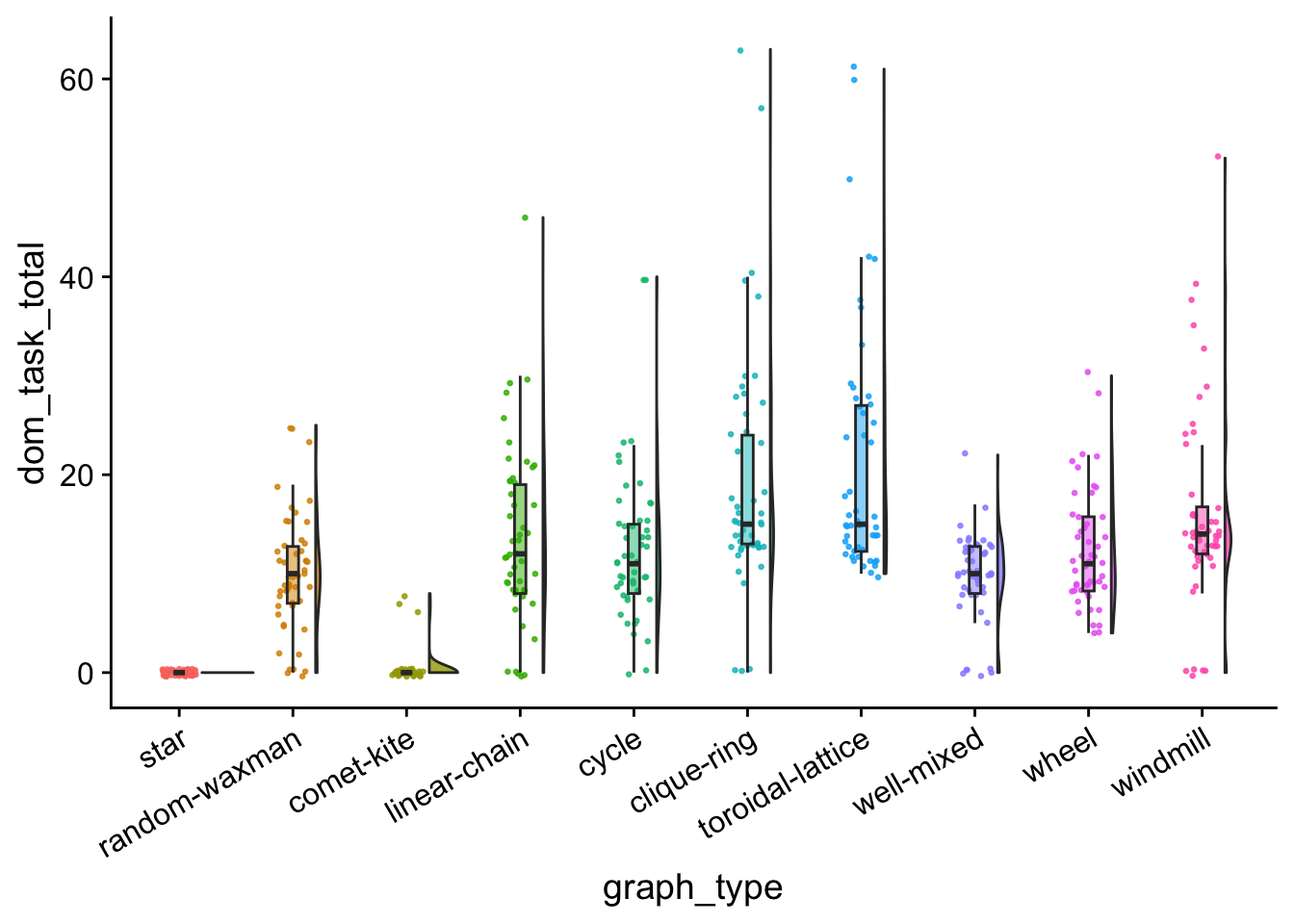
data %>%
  group_by(graph_type) %>%
  summarize(
    reps = n(),
    median_dom_task_total = median(dom_task_total),
    mean_dom_task_total = mean(dom_task_total)
  ) %>%
  arrange(
    desc(mean_dom_task_total)
  )
## # A tibble: 10 × 4
## graph_type reps median_dom_task_total mean_dom_task_total
## <fct> <int> <dbl> <dbl>
## 1 toroidal-lattice 50 15 21.4
## 2 clique-ring 50 15 19.2
## 3 windmill 50 14 16.1
## 4 linear-chain 50 12 13.6
## 5 cycle 50 11 12.6
## 6 wheel 50 11 12.4
## 7 random-waxman 50 10 9.92
## 8 well-mixed 50 10 9.62
## 9 comet-kite 50 0 0.42
## 10 star 50 0 0kruskal.test(
formula = dom_task_total ~ graph_type,
data = data
)##
## Kruskal-Wallis rank sum test
##
## data: dom_task_total by graph_type
## Kruskal-Wallis chi-squared = 262.43, df = 9, p-value < 2.2e-16wc_results <- pairwise.wilcox.test(
x = data$dom_task_total,
g = data$graph_type,
p.adjust.method = "holm",
exact = FALSE
)
dom_task_total_wc_table <- kbl(wc_results$p.value) %>% kable_styling()
save_kable(dom_task_total_wc_table, paste0(plot_dir, "/dom_task_total_wc_table.pdf"))
dom_task_total_wc_table| star | random-waxman | comet-kite | linear-chain | cycle | clique-ring | toroidal-lattice | well-mixed | wheel | |
|---|---|---|---|---|---|---|---|---|---|
| random-waxman | 0.0000000 | NA | NA | NA | NA | NA | NA | NA | NA |
| comet-kite | 0.9646146 | 0.0000000 | NA | NA | NA | NA | NA | NA | NA |
| linear-chain | 0.0000000 | 0.4710663 | 0 | NA | NA | NA | NA | NA | NA |
| cycle | 0.0000000 | 0.9646146 | 0 | 1.0000000 | NA | NA | NA | NA | NA |
| clique-ring | 0.0000000 | 0.0000042 | 0 | 0.0907079 | 0.0083936 | NA | NA | NA | NA |
| toroidal-lattice | 0.0000000 | 0.0000001 | 0 | 0.0112805 | 0.0003268 | 1.0000000 | NA | NA | NA |
| well-mixed | 0.0000000 | 1.0000000 | 0 | 0.5076566 | 0.9646146 | 0.0000000 | 0.0000000 | NA | NA |
| wheel | 0.0000000 | 0.9646146 | 0 | 1.0000000 | 1.0000000 | 0.0033520 | 0.0001346 | 0.9865397 | NA |
| windmill | 0.0000000 | 0.0009903 | 0 | 0.9865397 | 0.4321933 | 0.9865397 | 0.7677082 | 0.0000305 | 0.2316497 |
Tasks done by organisms not in dominant taxon:
data <- data %>%
  mutate(
    nondom_pop_task_prop = case_when(
      pop_task_total == 0 ~ 0,
      .default = (pop_task_total - dom_task_total) / (pop_task_total)
    )
  )

nondom_tasks_total_plt <- ggplot(
    data = data,
    mapping = aes(
      x = graph_type,
      y = nondom_pop_task_prop,
      fill = graph_type
    )
  ) +
  geom_flat_violin(
    position = position_nudge(x = .2, y = 0),
    alpha = .8
  ) +
  geom_point(
    mapping=aes(color = graph_type),
    position = position_jitter(width = .15),
    size = .5,
    alpha = 0.8
  ) +
  geom_boxplot(
    width = .1,
    outlier.shape = NA,
    alpha = 0.5
  ) +
  theme(
    legend.position = "none",
    axis.text.x = element_text(
      angle = 30,
      hjust = 1
    )
  )

ggsave(
  filename = paste0(plot_dir, "/non_dom_tasks_total.pdf"),
  plot = nondom_tasks_total_plt,
  width = 15,
  height = 10
)

nondom_tasks_total_plt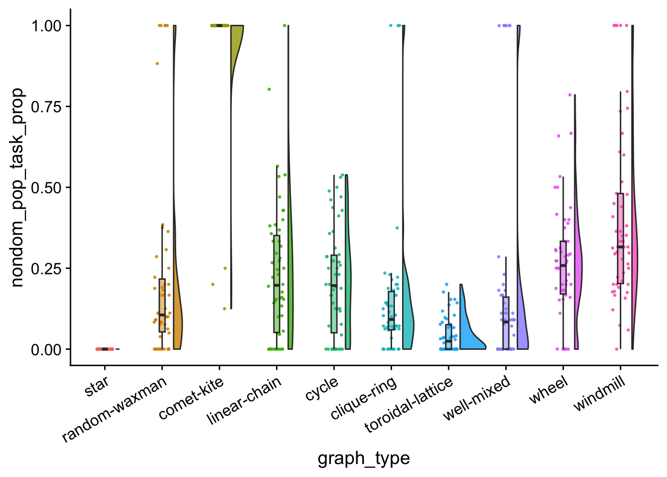
data %>%
  group_by(graph_type) %>%
  summarize(
    reps = n(),
    median_nondom_pop_task_prop = median(nondom_pop_task_prop),
    mean_nondom_pop_task_prop = mean(nondom_pop_task_prop)
  ) %>%
  arrange(
    desc(mean_nondom_pop_task_prop)
  )
## # A tibble: 10 × 4
## graph_type reps median_nondom_pop_task_prop mean_nondom_pop_task_prop
## <fct> <int> <dbl> <dbl>
## 1 comet-kite 50 1 0.952
## 2 windmill 50 0.316 0.398
## 3 wheel 50 0.258 0.264
## 4 linear-chain 50 0.197 0.234
## 5 random-waxman 50 0.106 0.222
## 6 cycle 50 0.196 0.206
## 7 well-mixed 50 0.0839 0.177
## 8 clique-ring 50 0.0917 0.154
## 9 toroidal-lattice 50 0.0245 0.0432
## 10 star 50 0 0kruskal.test(
formula = nondom_pop_task_prop ~ graph_type,
data = data
)##
## Kruskal-Wallis rank sum test
##
## data: nondom_pop_task_prop by graph_type
## Kruskal-Wallis chi-squared = 256.7, df = 9, p-value < 2.2e-16wc_results <- pairwise.wilcox.test(
x = data$nondom_pop_task_prop,
g = data$graph_type,
p.adjust.method = "holm",
exact = FALSE
)
nondom_pop_task_prop_wc_table <- kbl(wc_results$p.value) %>% kable_styling()
save_kable(nondom_pop_task_prop_wc_table, paste0(plot_dir, "/nondom_pop_task_prop_wc_table.pdf"))
nondom_pop_task_prop_wc_table| star | random-waxman | comet-kite | linear-chain | cycle | clique-ring | toroidal-lattice | well-mixed | wheel | |
|---|---|---|---|---|---|---|---|---|---|
| random-waxman | 0e+00 | NA | NA | NA | NA | NA | NA | NA | NA |
| comet-kite | 0e+00 | 0.0000000 | NA | NA | NA | NA | NA | NA | NA |
| linear-chain | 0e+00 | 0.9560919 | 0 | NA | NA | NA | NA | NA | NA |
| cycle | 0e+00 | 1.0000000 | 0 | 1.0000000 | NA | NA | NA | NA | NA |
| clique-ring | 0e+00 | 1.0000000 | 0 | 0.1142983 | 0.1337364 | NA | NA | NA | NA |
| toroidal-lattice | 2e-07 | 0.0001655 | 0 | 0.0000044 | 0.0000102 | 0.0019354 | NA | NA | NA |
| well-mixed | 0e+00 | 0.4737074 | 0 | 0.0370381 | 0.0501364 | 1.0000000 | 0.4737074 | NA | NA |
| wheel | 0e+00 | 0.0560536 | 0 | 1.0000000 | 0.8350382 | 0.0002916 | 0.0000000 | 0.0003351 | NA |
| windmill | 0e+00 | 0.0000660 | 0 | 0.0129065 | 0.0022312 | 0.0000000 | 0.0000000 | 0.0000002 | 0.1337364 |
# kruskal.test(
#   formula = dom_task_total ~ graph_type,
#   data = filter(completed_runs_data)
# )
6.4 Dominant gestation time
dom_gestation_time_plt <- ggplot(
    data = data,
    mapping = aes(
      x = graph_type,
      y = dom_detail_gestation_time,
      fill = graph_type
    )
  ) +
  geom_flat_violin(
    position = position_nudge(x = .2, y = 0),
    alpha = .8
  ) +
  geom_point(
    mapping=aes(color = graph_type),
    position = position_jitter(width = .15),
    size = .5,
    alpha = 0.8
  ) +
  geom_boxplot(
    width = .1,
    outlier.shape = NA,
    alpha = 0.5
  ) +
  theme(
    legend.position = "none",
    axis.text.x = element_text(
      angle = 30,
      hjust = 1
    )
  )

ggsave(
  filename = paste0(plot_dir, "/dom_gestation_time.pdf"),
  plot = dom_gestation_time_plt,
  width = 15,
  height = 10
)

dom_gestation_time_plt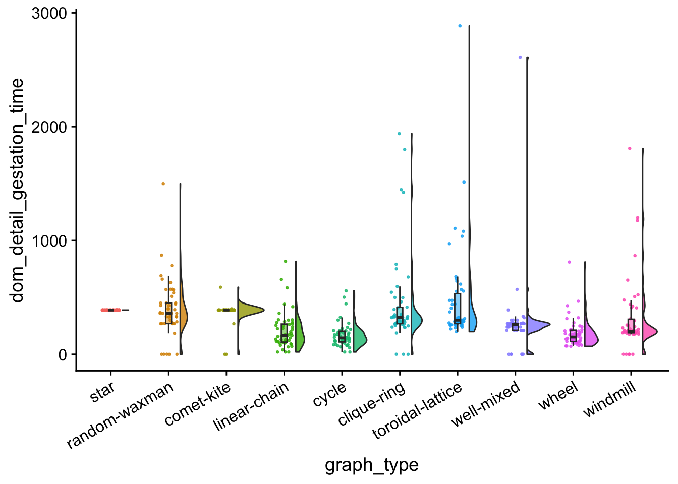
data %>%
  group_by(graph_type) %>%
  summarize(
    reps = n(),
    median_dom_detail_gestation_time = median(dom_detail_gestation_time),
    mean_dom_detail_gestation_time = mean(dom_detail_gestation_time)
  ) %>%
  arrange(
    desc(mean_dom_detail_gestation_time)
  )
## # A tibble: 10 × 4
## graph_type reps median_dom_detail_gestation_t…¹ mean_dom_detail_gest…²
## <fct> <int> <dbl> <dbl>
## 1 toroidal-lattice 50 300. 480.
## 2 clique-ring 50 324. 440.
## 3 random-waxman 50 360 393.
## 4 star 50 389 389
## 5 comet-kite 50 389 375.
## 6 windmill 50 204. 315.
## 7 well-mixed 50 260. 281.
## 8 linear-chain 50 164 208.
## 9 wheel 50 152. 187.
## 10 cycle 50 144. 169.
## # ℹ abbreviated names: ¹median_dom_detail_gestation_time,
## # ²mean_dom_detail_gestation_timekruskal.test(
formula = dom_detail_gestation_time ~ graph_type,
data = data
)##
## Kruskal-Wallis rank sum test
##
## data: dom_detail_gestation_time by graph_type
## Kruskal-Wallis chi-squared = 197.97, df = 9, p-value < 2.2e-16wc_results <- pairwise.wilcox.test(
x = data$dom_detail_gestation_time,
g = data$graph_type,
p.adjust.method = "holm",
exact = FALSE
)
dom_detail_gestation_time_wc_table <- kbl(wc_results$p.value) %>% kable_styling()
save_kable(dom_detail_gestation_time_wc_table, paste0(plot_dir, "/dom_detail_gestation_time_wc_table.pdf"))
dom_detail_gestation_time_wc_table| star | random-waxman | comet-kite | linear-chain | cycle | clique-ring | toroidal-lattice | well-mixed | wheel | |
|---|---|---|---|---|---|---|---|---|---|
| random-waxman | 1.0000000 | NA | NA | NA | NA | NA | NA | NA | NA |
| comet-kite | 1.0000000 | 1.0000000 | NA | NA | NA | NA | NA | NA | NA |
| linear-chain | 0.0000000 | 0.0000161 | 0.0000000 | NA | NA | NA | NA | NA | NA |
| cycle | 0.0000000 | 0.0000001 | 0.0000000 | 1.0000000 | NA | NA | NA | NA | NA |
| clique-ring | 0.0039456 | 1.0000000 | 0.0375642 | 0.0000080 | 0.0000000 | NA | NA | NA | NA |
| toroidal-lattice | 0.1400273 | 1.0000000 | 0.5320337 | 0.0000001 | 0.0000000 | 1.0000000 | NA | NA | NA |
| well-mixed | 0.0000000 | 0.0000135 | 0.0000000 | 0.1875321 | 0.0000565 | 0.0001086 | 1.61e-05 | NA | NA |
| wheel | 0.0000000 | 0.0000003 | 0.0000000 | 1.0000000 | 1.0000000 | 0.0000000 | 0.00e+00 | 0.0012044 | NA |
| windmill | 0.0000430 | 0.0038095 | 0.0005370 | 0.2673588 | 0.0015818 | 0.0015818 | 4.30e-05 | 0.5320337 | 0.0088282 |
6.5 Dominant genome length
dom_genome_length_plt <- ggplot(
    data = data,
    mapping = aes(
      x = graph_type,
      y = dom_detail_genome_length,
      fill = graph_type
    )
  ) +
  geom_flat_violin(
    position = position_nudge(x = .2, y = 0),
    alpha = .8
  ) +
  geom_point(
    mapping=aes(color = graph_type),
    position = position_jitter(width = .15),
    size = .5,
    alpha = 0.8
  ) +
  geom_boxplot(
    width = .1,
    outlier.shape = NA,
    alpha = 0.5
  ) +
  theme(
    legend.position = "none",
    axis.text.x = element_text(
      angle = 30,
      hjust = 1
    )
  )

ggsave(
  filename = paste0(plot_dir, "/dom_genome_length.pdf"),
  plot = dom_genome_length_plt,
  width = 15,
  height = 10
)

dom_genome_length_plt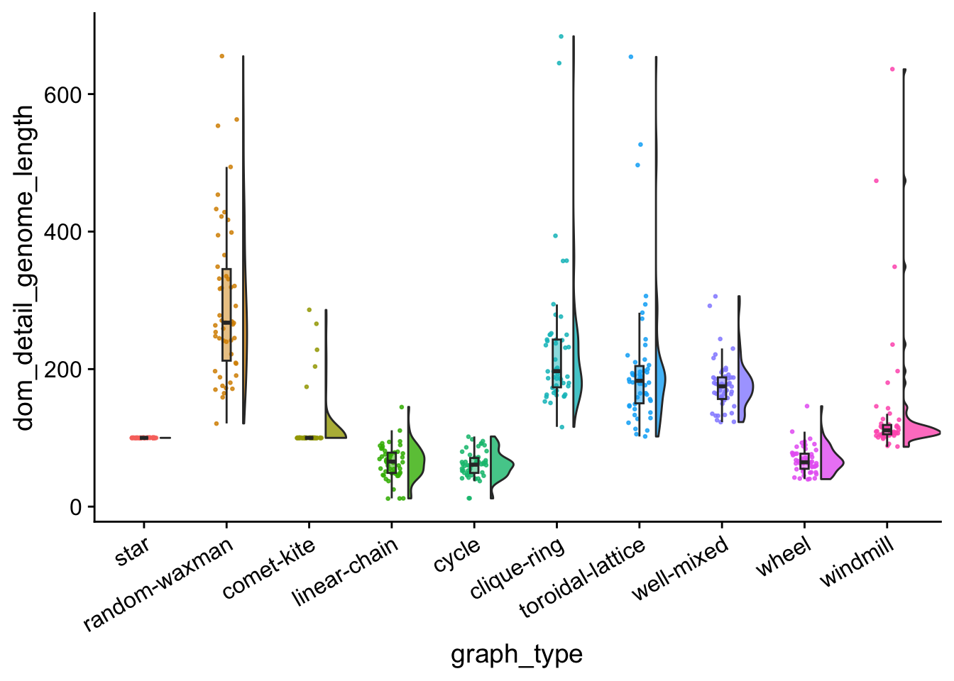
data %>%
  group_by(graph_type) %>%
  summarize(
    reps = n(),
    median_dom_detail_genome_length = median(dom_detail_genome_length),
    mean_dom_detail_genome_length = mean(dom_detail_genome_length)
  ) %>%
  arrange(
    desc(mean_dom_detail_genome_length)
  )
## # A tibble: 10 × 4
## graph_type reps median_dom_detail_genome_length mean_dom_detail_geno…¹
## <fct> <int> <dbl> <dbl>
## 1 random-waxman 50 268. 298.
## 2 clique-ring 50 197 230.
## 3 toroidal-lattice 50 183 203.
## 4 well-mixed 50 175 177.
## 5 windmill 50 111 139.
## 6 comet-kite 50 100 113.
## 7 star 50 100 100
## 8 wheel 50 64.5 68.2
## 9 linear-chain 50 65.5 64.4
## 10 cycle 50 61 61.2
## # ℹ abbreviated name: ¹mean_dom_detail_genome_lengthkruskal.test(
formula = dom_detail_genome_length ~ graph_type,
data = data
)##
## Kruskal-Wallis rank sum test
##
## data: dom_detail_genome_length by graph_type
## Kruskal-Wallis chi-squared = 423.75, df = 9, p-value < 2.2e-16wc_results <- pairwise.wilcox.test(
x = data$dom_detail_genome_length,
g = data$graph_type,
p.adjust.method = "holm",
exact = FALSE
)
dom_detail_genome_length_wc_table <- kbl(wc_results$p.value) %>% kable_styling()
save_kable(dom_detail_genome_length_wc_table, paste0(plot_dir, "/dom_detail_genome_length_wc_table.pdf"))
dom_detail_genome_length_wc_table| star | random-waxman | comet-kite | linear-chain | cycle | clique-ring | toroidal-lattice | well-mixed | wheel | |
|---|---|---|---|---|---|---|---|---|---|
| random-waxman | 0.0000000 | NA | NA | NA | NA | NA | NA | NA | NA |
| comet-kite | 0.1373564 | 0.0000000 | NA | NA | NA | NA | NA | NA | NA |
| linear-chain | 0.0000000 | 0.0000000 | 0 | NA | NA | NA | NA | NA | NA |
| cycle | 0.0000000 | 0.0000000 | 0 | 0.85562 | NA | NA | NA | NA | NA |
| clique-ring | 0.0000000 | 0.0007957 | 0 | 0.00000 | 0.0000000 | NA | NA | NA | NA |
| toroidal-lattice | 0.0000000 | 0.0000044 | 0 | 0.00000 | 0.0000000 | 0.1373564 | NA | NA | NA |
| well-mixed | 0.0000000 | 0.0000000 | 0 | 0.00000 | 0.0000000 | 0.0016198 | 0.85562 | NA | NA |
| wheel | 0.0000000 | 0.0000000 | 0 | 0.85562 | 0.4828684 | 0.0000000 | 0.00000 | 0 | NA |
| windmill | 0.0000000 | 0.0000000 | 0 | 0.00000 | 0.0000000 | 0.0000000 | 0.00000 | 0 | 0 |
6.6 Task profile entropy
task_profile_entropy_plt <- ggplot(
    data = data,
    mapping = aes(
      x = graph_type,
      y = task_profile_entropy,
      fill = graph_type
    )
  ) +
  geom_flat_violin(
    position = position_nudge(x = .2, y = 0),
    alpha = .8
  ) +
  geom_point(
    mapping=aes(color = graph_type),
    position = position_jitter(width = .15),
    size = .5,
    alpha = 0.8
  ) +
  geom_boxplot(
    width = .1,
    outlier.shape = NA,
    alpha = 0.5
  ) +
  theme(
    legend.position = "none",
    axis.text.x = element_text(
      angle = 30,
      hjust = 1
    )
  )

ggsave(
  filename = paste0(plot_dir, "/task_profile_entropy.pdf"),
  plot = task_profile_entropy_plt,
  width = 15,
  height = 10
)

task_profile_entropy_plt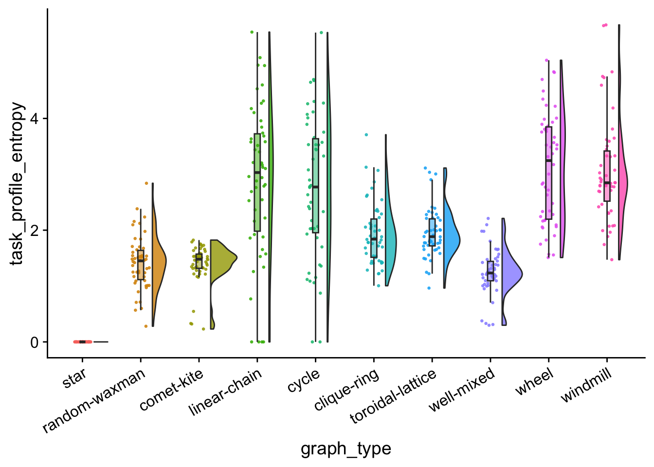
task_profile_count_plt <- ggplot(
    data = data,
    mapping = aes(
      x = graph_type,
      y = task_profile_count,
      fill = graph_type
    )
  ) +
  geom_flat_violin(
    position = position_nudge(x = .2, y = 0),
    alpha = .8
  ) +
  geom_point(
    mapping=aes(color = graph_type),
    position = position_jitter(width = .15),
    size = .5,
    alpha = 0.8
  ) +
  geom_boxplot(
    width = .1,
    outlier.shape = NA,
    alpha = 0.5
  ) +
  theme(
    legend.position = "none",
    axis.text.x = element_text(
      angle = 30,
      hjust = 1
    )
  )

ggsave(
  filename = paste0(plot_dir, "/task_profile_count.pdf"),
  plot = task_profile_count_plt,
  width = 15,
  height = 10
)

task_profile_count_plt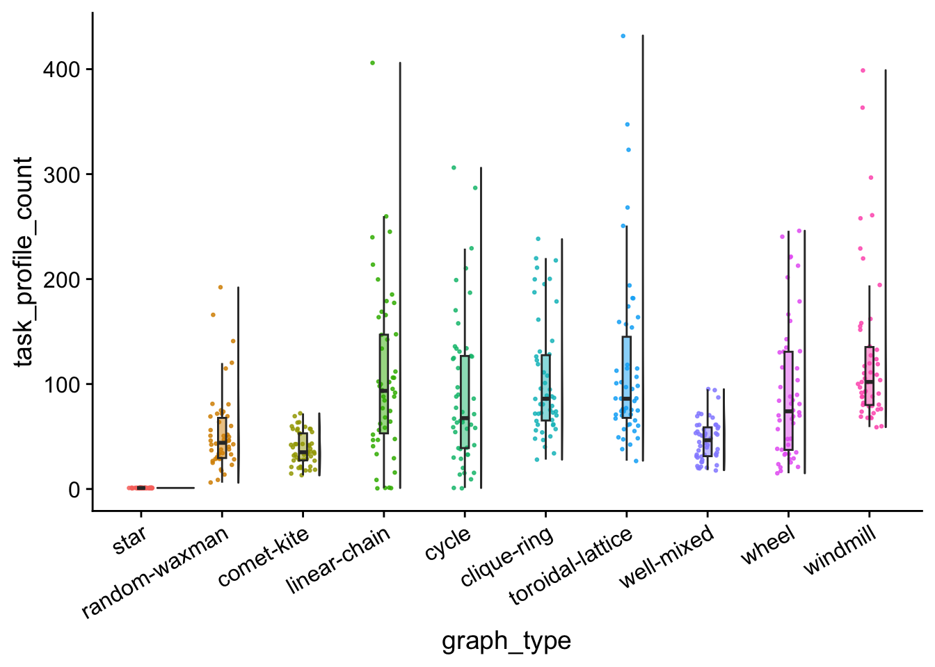
6.7 Average generation
avg_generation_plt <- ggplot(
    data = data,
    mapping = aes(
      x = graph_type,
      y = time_average_generation,
      fill = graph_type
    )
  ) +
  geom_flat_violin(
    position = position_nudge(x = .2, y = 0),
    alpha = .8
  ) +
  geom_point(
    mapping=aes(color = graph_type),
    position = position_jitter(width = .15),
    size = .5,
    alpha = 0.8
  ) +
  geom_boxplot(
    width = .1,
    outlier.shape = NA,
    alpha = 0.5
  ) +
  theme(
    legend.position = "none",
    axis.text.x = element_text(
      angle = 30,
      hjust = 1
    )
  )

ggsave(
  filename = paste0(plot_dir, "/avg_generation.pdf"),
  plot = avg_generation_plt,
  width = 15,
  height = 10
)

avg_generation_plt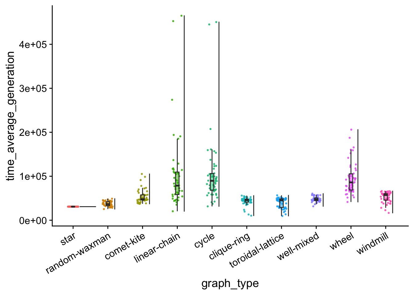
6.8 Population task count over time
pop_task_cnt_ts <- ggplot(
    data = time_series_data,
    mapping = aes(
      x = update,
      y = pop_task_total_tasks_done,
      color = graph_type,
      fill = graph_type
    )
  ) +
  stat_summary(fun = "mean", geom = "line") +
  stat_summary(
    fun.data = "mean_cl_boot",
    fun.args = list(conf.int = 0.95),
    geom = "ribbon",
    alpha = 0.2,
    linetype = 0
  ) +
  theme(legend.position = "bottom")

ggsave(
  plot = pop_task_cnt_ts,
  filename = paste0(
    working_directory,
    "/plots/pop_tasks_ts.pdf"
  ),
  width = 15,
  height = 10
)

pop_task_cnt_ts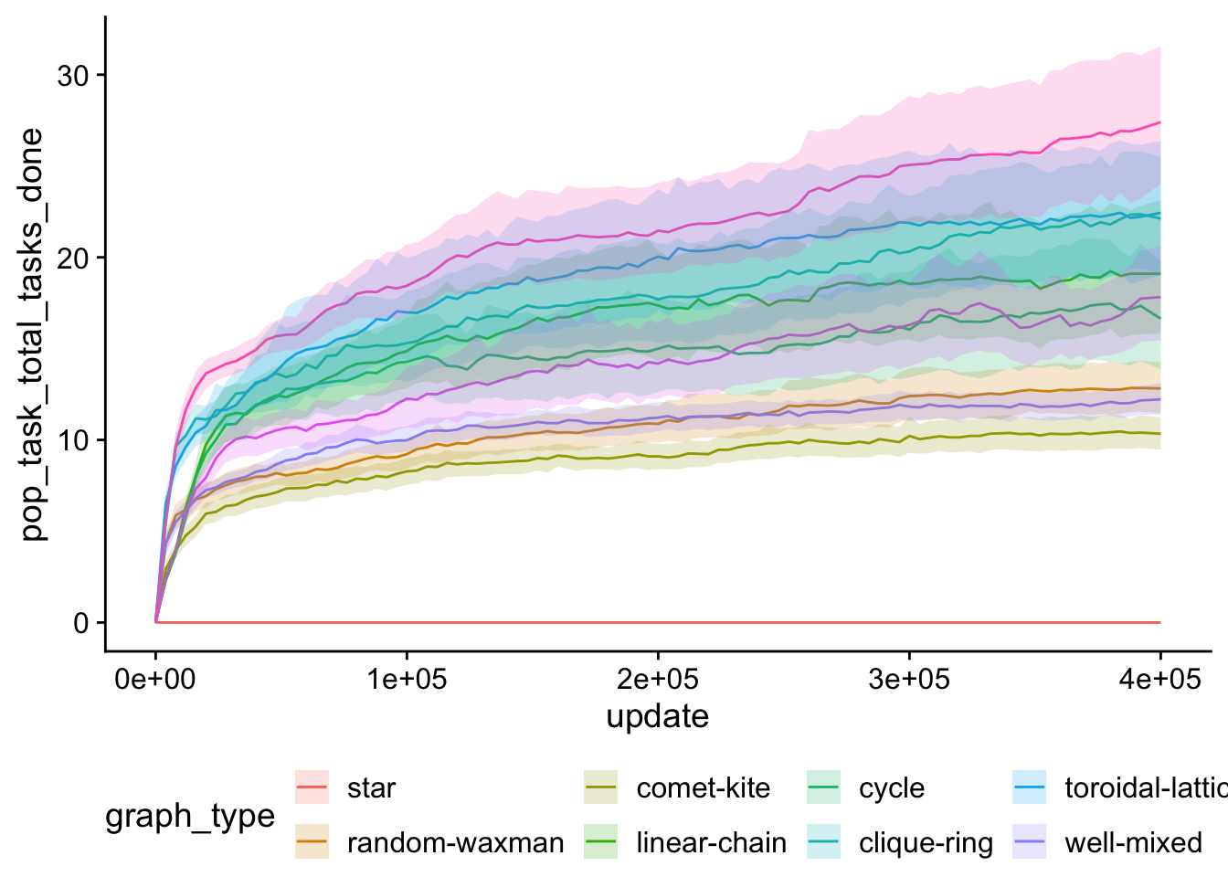
6.9 Average generation over time
time_average_generation_ts <- ggplot(
    data = time_series_data,
    mapping = aes(
      x = update,
      y = time_average_generation,
      color = graph_type,
      fill = graph_type
    )
  ) +
  stat_summary(fun = "mean", geom = "line") +
  stat_summary(
    fun.data = "mean_cl_boot",
    fun.args = list(conf.int = 0.95),
    geom = "ribbon",
    alpha = 0.2,
    linetype = 0
  ) +
  facet_wrap(~ENVIRONMENT_FILE) +
  theme(legend.position = "bottom")

ggsave(
  plot = time_average_generation_ts,
  filename = paste0(
    working_directory,
    "/plots/time_average_generation_ts.pdf"
  ),
  width = 15,
  height = 10
)

time_average_generation_ts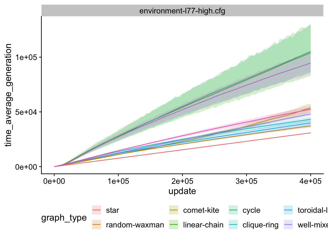
6.10 Graph location info
Analyze graph_birth_info_annotated.csv
# Load summary data from final update
graph_loc_data_path <- paste(
  working_directory,
  "data",
  "graph_birth_info_annotated.csv",
  sep = "/"
)
graph_loc_data <- read_csv(graph_loc_data_path)

graph_loc_data <- graph_loc_data %>%
  mutate(
    graph_type = factor(
      graph_type,
      levels = c(
        "star",
        "random-waxman",
        "comet-kite",
        "linear-chain",
        "cycle",
        "clique-ring",
        "toroidal-lattice",
        "well-mixed",
        "wheel",
        "windmill"
      )
    ),
    seed = as.factor(seed)
  ) %>%
  filter(
    graph_type %in% focal_graphs
  )
Summarize by seed
graph_loc_data_summary <- graph_loc_data %>%
  group_by(seed, graph_type) %>%
  summarize(
    births_var = var(births),
    births_total = sum(births),
    task_apps_total = sum(task_appearances),
    task_apps_var = var(task_appearances)
  ) %>%
  ungroup()
6.10.1 Total birth Counts
birth_counts_total_plt <- ggplot(
    data = graph_loc_data_summary,
    mapping = aes(
      x = graph_type,
      y = births_total,
      fill = graph_type
    )
  ) +
  geom_flat_violin(
    position = position_nudge(x = .2, y = 0),
    alpha = .8
  ) +
  geom_point(
    mapping=aes(color = graph_type),
    position = position_jitter(width = .15),
    size = .5,
    alpha = 0.8
  ) +
  geom_boxplot(
    width = .1,
    outlier.shape = NA,
    alpha = 0.5
  ) +
  theme(
    legend.position = "none",
    axis.text.x = element_text(
      angle = 30,
      hjust = 1
    )
  )

ggsave(
  filename = paste0(plot_dir, "/birth_counts_total.pdf"),
  plot = birth_counts_total_plt,
  width = 15,
  height = 10
)

birth_counts_total_plt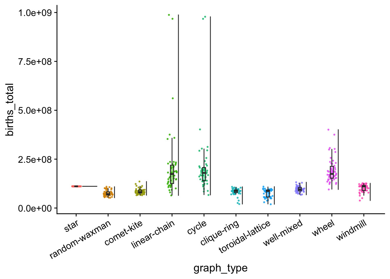
6.10.2 Variance birth Counts
birth_counts_var_plt <- ggplot(
    data = graph_loc_data_summary,
    mapping = aes(
      x = graph_type,
      y = births_var,
      fill = graph_type
    )
  ) +
  geom_flat_violin(
    position = position_nudge(x = .2, y = 0),
    alpha = .8
  ) +
  geom_point(
    mapping=aes(color = graph_type),
    position = position_jitter(width = .15),
    size = .5,
    alpha = 0.8
  ) +
  geom_boxplot(
    width = .1,
    outlier.shape = NA,
    alpha = 0.5
  ) +
  theme(
    legend.position = "none",
    axis.text.x = element_text(
      angle = 30,
      hjust = 1
    )
  )

ggsave(
  filename = paste0(plot_dir, "/birth_counts_var.pdf"),
  plot = birth_counts_var_plt,
  width = 15,
  height = 10
)

birth_counts_var_plt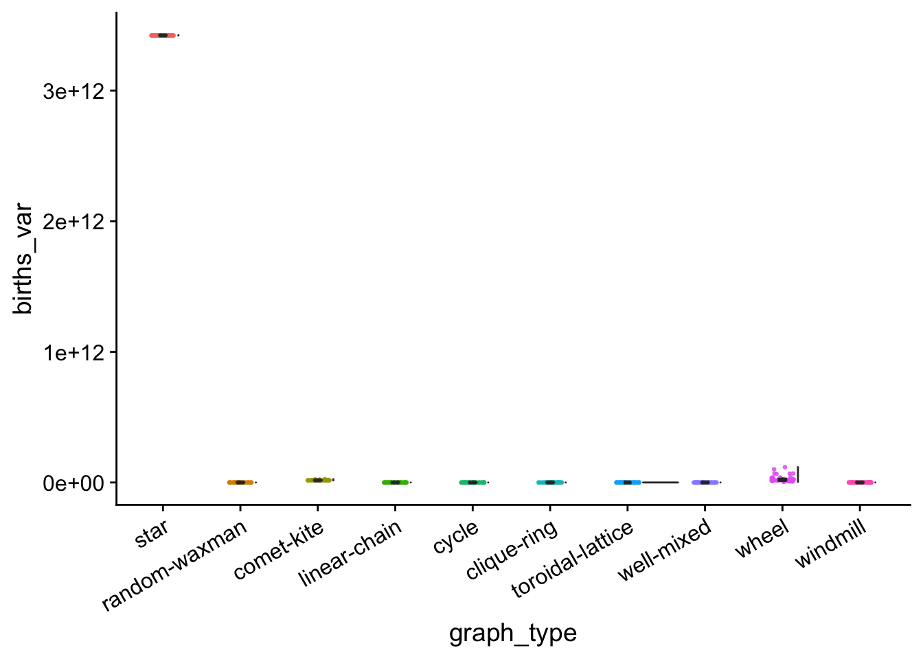
6.10.3 Task appearances total
task_apps_total_plt <- ggplot(
    data = graph_loc_data_summary,
    mapping = aes(
      x = graph_type,
      y = task_apps_total,
      fill = graph_type
    )
  ) +
  geom_flat_violin(
    position = position_nudge(x = .2, y = 0),
    alpha = .8
  ) +
  geom_point(
    mapping=aes(color = graph_type),
    position = position_jitter(width = .15),
    size = .5,
    alpha = 0.8
  ) +
  geom_boxplot(
    width = .1,
    outlier.shape = NA,
    alpha = 0.5
  ) +
  theme(
    legend.position = "none",
    axis.text.x = element_text(
      angle = 30,
      hjust = 1
    )
  )

ggsave(
  filename = paste0(plot_dir, "/task_apps_total.pdf"),
  plot = task_apps_total_plt,
  width = 15,
  height = 10
)

task_apps_total_plt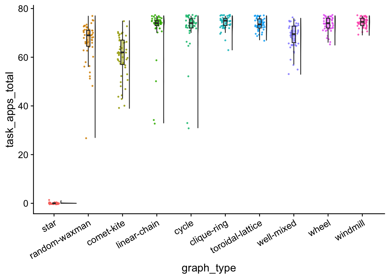
kruskal.test(
  formula = task_apps_total ~ graph_type,
  data = graph_loc_data_summary
)
##
## Kruskal-Wallis rank sum test
##
## data: task_apps_total by graph_type
## Kruskal-Wallis chi-squared = 288.67, df = 9, p-value < 2.2e-16wc_results <- pairwise.wilcox.test(
x = graph_loc_data_summary$task_apps_total,
g = graph_loc_data_summary$graph_type,
p.adjust.method = "holm",
exact = FALSE
)
wc_results##
## Pairwise comparisons using Wilcoxon rank sum test with continuity correction
##
## data: graph_loc_data_summary$task_apps_total and graph_loc_data_summary$graph_type
##
## star random-waxman comet-kite linear-chain cycle
## random-waxman < 2e-16 - - - -
## comet-kite < 2e-16 0.00089 - - -
## linear-chain < 2e-16 2.8e-08 2.7e-11 - -
## cycle < 2e-16 8.3e-07 6.3e-11 1.00000 -
## clique-ring < 2e-16 4.4e-10 2.0e-14 1.00000 1.00000
## toroidal-lattice < 2e-16 1.2e-08 3.7e-14 1.00000 1.00000
## well-mixed < 2e-16 1.00000 3.5e-06 8.8e-07 2.1e-05
## wheel < 2e-16 1.4e-08 8.1e-14 1.00000 1.00000
## windmill < 2e-16 2.7e-11 4.3e-15 1.00000 1.00000
## clique-ring toroidal-lattice well-mixed wheel
## random-waxman - - - -
## comet-kite - - - -
## linear-chain - - - -
## cycle - - - -
## clique-ring - - - -
## toroidal-lattice 1.00000 - - -
## well-mixed 2.3e-08 7.7e-07 - -
## wheel 1.00000 1.00000 5.0e-07 -
## windmill 1.00000 1.00000 1.2e-09 1.00000
##
## P value adjustment method: holm