Chapter 7 Multi-path exploration diagnostic

experiment_slug <- "2023-12-28-phylo-sampling-diag"

working_directory <- paste0(
  "experiments/",
  experiment_slug,
  "/analysis/"
)

if (exists("bookdown_wd_prefix")) {
  working_directory <- paste0(
    bookdown_wd_prefix,
    working_directory
  )
}

7.1 Dependencies

library(tidyverse)
library(cowplot)
library(RColorBrewer)
library(khroma)
library(rstatix)
library(knitr)
source("https://gist.githubusercontent.com/benmarwick/2a1bb0133ff568cbe28d/raw/fb53bd97121f7f9ce947837ef1a4c65a73bffb3f/geom_flat_violin.R")

print(version)

##                _                           
## platform       aarch64-apple-darwin20      
## arch           aarch64                     
## os             darwin20                    
## system         aarch64, darwin20           
## status                                     
## major          4                           
## minor          2.1                         
## year           2022                        
## month          06                          
## day            23                          
## svn rev        82513                       
## language       R                           
## version.string R version 4.2.1 (2022-06-23)
## nickname       Funny-Looking Kid

7.2 Setup

# Configure our default graphing theme
theme_set(theme_cowplot())
# Create a directory to store plots
plot_directory <- paste0(working_directory, "plots/")
dir.create(plot_directory, showWarnings=FALSE)
# Constants
focal_diagnostic <- "multipath-exploration"

7.2.1 Load experiment summary data

summary_data_loc <- paste0(working_directory, "data/aggregate.csv")
summary_data <- read_csv(summary_data_loc)

## Rows: 1080 Columns: 58
## ── Column specification ───────────────────────────────────────────────────────────────────────────────────────────────────────────────────────────────────────────
## Delimiter: ","
## chr  (5): DIAGNOSTIC, EVAL_FIT_EST_MODE, EVAL_MODE, SELECTION, STOP_MODE
## dbl (53): ACCURACY, CREDIT, DIAGNOSTIC_DIMENSIONALITY, EVAL_MAX_PHYLO_SEARCH...
## 
## ℹ Use `spec()` to retrieve the full column specification for this data.
## ℹ Specify the column types or set `show_col_types = FALSE` to quiet this message.

summary_data <- summary_data %>%
  mutate(
    evals_per_gen = case_when(
      EVAL_MODE == "cohort-full-compete" ~ 1.0 / NUM_COHORTS,
      EVAL_MODE == "cohort" ~ 1.0 / NUM_COHORTS,
      EVAL_MODE == "down-sample" ~ TEST_DOWNSAMPLE_RATE,
      EVAL_MODE == "full" ~ 1.0,
      EVAL_MODE == "indiv-rand-sample" ~ TEST_DOWNSAMPLE_RATE,
      EVAL_MODE == "phylo-informed-sample" ~ TEST_DOWNSAMPLE_RATE
    ),
    EVAL_FIT_EST_MODE = case_when(
      EVAL_FIT_EST_MODE == "ancestor-opt" ~ "ancestor",
      EVAL_FIT_EST_MODE == "relative-opt" ~ "relative",
      .default = EVAL_FIT_EST_MODE
    ),
    .keep = "all"
  ) %>%
  mutate(
    eval_label = case_when(
      # Clean up down-sample label
      EVAL_MODE == "down-sample" & EVAL_FIT_EST_MODE != "none" ~ paste("down-sample", EVAL_FIT_EST_MODE, sep="-"),
      .default = EVAL_MODE
    ),
  ) %>%
  mutate(
    evals_per_gen = as.factor(evals_per_gen),
    DIAGNOSTIC = as.factor(DIAGNOSTIC),
    SELECTION = as.factor(SELECTION),
    EVAL_MODE = as.factor(EVAL_MODE),
    NUM_COHORTS = as.factor(NUM_COHORTS),
    TEST_DOWNSAMPLE_RATE = as.factor(TEST_DOWNSAMPLE_RATE),
    EVAL_FIT_EST_MODE = factor(
      EVAL_FIT_EST_MODE,
      levels = c(
        "none",
        "ancestor",
        "relative"
      ),
      labels = c(
        "None",
        "Ancestor",
        "Relative"
      )
    )
  )

explore_summary_data <- filter(
  summary_data,
  DIAGNOSTIC == "multipath-exploration"
)

7.2.2 Load experiment time series data

ts_data_loc <- paste0(working_directory, "data/time_series.csv")
ts_data <- read_csv(ts_data_loc)

## Rows: 108000 Columns: 28
## ── Column specification ───────────────────────────────────────────────────────────────────────────────────────────────────────────────────────────────────────────
## Delimiter: ","
## chr  (4): DIAGNOSTIC, EVAL_FIT_EST_MODE, EVAL_MODE, SELECTION
## dbl (24): NUM_COHORTS, SEED, TEST_DOWNSAMPLE_RATE, ave_depth, deleterious_st...
## 
## ℹ Use `spec()` to retrieve the full column specification for this data.
## ℹ Specify the column types or set `show_col_types = FALSE` to quiet this message.

ts_data <- ts_data %>%
  mutate(
    evals_per_gen = case_when(
      EVAL_MODE == "cohort-full-compete" ~ 1.0 / NUM_COHORTS,
      EVAL_MODE == "cohort" ~ 1.0 / NUM_COHORTS,
      EVAL_MODE == "down-sample" ~ TEST_DOWNSAMPLE_RATE,
      EVAL_MODE == "full" ~ 1.0,
      EVAL_MODE == "indiv-rand-sample" ~ TEST_DOWNSAMPLE_RATE,
      EVAL_MODE == "phylo-informed-sample" ~ TEST_DOWNSAMPLE_RATE
    ),
    EVAL_FIT_EST_MODE = case_when(
      EVAL_FIT_EST_MODE == "ancestor-opt" ~ "ancestor",
      EVAL_FIT_EST_MODE == "relative-opt" ~ "relative",
      .default = EVAL_FIT_EST_MODE
    ),
    .keep = "all"
  ) %>%
  mutate(
    eval_label = case_when(
      EVAL_MODE == "down-sample" & EVAL_FIT_EST_MODE != "none" ~ paste("down-sample", EVAL_FIT_EST_MODE, sep="-"),
      .default = EVAL_MODE
    )
  ) %>%
  mutate(
    evals_per_gen = as.factor(evals_per_gen),
    DIAGNOSTIC = as.factor(DIAGNOSTIC),
    SELECTION = as.factor(SELECTION),
    EVAL_MODE = as.factor(EVAL_MODE),
    NUM_COHORTS = as.factor(NUM_COHORTS),
    TEST_DOWNSAMPLE_RATE = as.factor(TEST_DOWNSAMPLE_RATE),
    EVAL_FIT_EST_MODE = factor(
      EVAL_FIT_EST_MODE,
      levels = c(
        "none",
        "ancestor",
        "relative"
      ),
      labels = c(
        "None",
        "Ancestor",
        "Relative"
      )
    )
  )

explore_ts_data <- ts_data %>%
  filter(DIAGNOSTIC == "multipath-exploration")

Summarize time series data

ts_summary_data <- ts_data %>%
  group_by(SEED, DIAGNOSTIC, SELECTION, evals_per_gen, eval_label) %>%
  summarize(
    n = n(),
    avg_num_unique_selected = mean(num_unique_selected),
    total_optimal_trait_coverage_loss = sum(optimal_trait_coverage_loss)
  )

## `summarise()` has grouped output by 'SEED', 'DIAGNOSTIC', 'SELECTION',
## 'evals_per_gen'. You can override using the `.groups` argument.

7.2.3 Plotting helper functions

The following function assist with exploratory plotting of different measurements from summary and time series data. Note that for these plots, standard lexicase reference is rendered at equivalent number of generations (instead of evaluations).

build_plot_summary_data <- function(data, diagnostic, selection, response) {
  diag_data <- data %>% filter(DIAGNOSTIC == diagnostic)

  full_median <- median(
    filter(
      diag_data,
      eval_label == "full" & SELECTION == selection
    )[[response]]
  )

  plot <- diag_data %>%
    filter(
      eval_label != "full" & SELECTION == selection
    ) %>%
    ggplot(
      aes_string(
        x = "eval_label",
        y = response,
        fill = "eval_label"
      )
    ) +
    geom_hline(
      yintercept = full_median,
      size = 1.0,
      alpha = 0.7,
      color = "black",
      linetype="dashed"
    ) +
    geom_flat_violin(
      position = position_nudge(x = .2, y = 0),
      alpha = .8,
      adjust = 1.5
    ) +
    geom_point(
      mapping = aes(color = eval_label),
      position = position_jitter(width = .15),
      size = .5,
      alpha = 0.8
    ) +
    geom_boxplot(
      width = .1,
      outlier.shape = NA,
      alpha = 0.5
    ) +
    scale_y_continuous(
      # limits = c(-0.5, 100)
    ) +
    scale_fill_bright() +
    scale_color_bright() +
    facet_grid(
      SELECTION ~ evals_per_gen,
      # nrow=2,
      labeller = label_both
    ) +
    theme(
      legend.position = "none",
      axis.text.x = element_text(
        angle = 30,
        hjust = 1
      ),
      panel.border = element_rect(color = "gray", size = 2)
    )

  return(plot)
}

build_plot_time_series_single_sampling <- function(
  data,
  diagnostic,
  selection,
  sampling_level,
  response
) {

  diag_data <- data %>% filter(
    DIAGNOSTIC == diagnostic &
    SELECTION == selection &
    evals_per_gen == sampling_level
  ) %>%
  mutate(
    sampling_level_label = sampling_level
  )

  full_diag_data <- data %>% filter(
    DIAGNOSTIC == diagnostic & SELECTION == selection & eval_label == "full"
  ) %>%
  mutate(
    # Ensure that median line will sit in same facet
    sampling_level_label = sampling_level
  )

  plot <- diag_data %>%
    filter(
      eval_label != "full"
    ) %>%
    ggplot(
      aes_string(
        x = "ts_step",
        # x = "evaluations",
        y = {{ response }}
      )
    ) +
    stat_summary(
      geom = "line",
      fun = mean,
      aes(
        color = eval_label
      )
    ) +
    stat_summary(
      geom = "ribbon",
      fun.data = "mean_cl_boot",
      fun.args = list(conf.int = 0.95),
      alpha = 0.2,
      linetype = 0,
      aes(
        color = eval_label,
        fill = eval_label
      )
    ) +
    scale_fill_bright() +
    scale_color_bright() +
    # facet_wrap(
    #   ~ sampling_level_label,
    #   ncol = 1,
    #   labeller = label_both
    # ) +
    theme(
      legend.position = "right"
    ) +
    stat_summary(
      data = full_diag_data,
      geom = "line",
      fun = median,
      linetype = "dashed",
      color = "black"
    )

  return(plot)
}

build_plot_time_series <- function(
  data,
  diagnostic,
  selection,
  response
) {
  # Build 1% sampling plot and 10% sampling plot
  p_01 <- data  %>% build_plot_time_series_single_sampling(
    diagnostic,
    selection,
    "0.01",
    response
  )
  p_10 <- data %>% build_plot_time_series_single_sampling(
    diagnostic,
    selection,
    "0.1",
    response
  )

  title <- ggdraw() +
    draw_label(
      paste0(diagnostic, " - ", selection),
      fontface = 'bold',
      x = 0,
      hjust = 0
    ) +
    theme(
      # add margin on the left of the drawing canvas,
      # so title is aligned with left edge of first plot
      plot.margin = margin(0, 0, 0, 7)
    )

  plot <- plot_grid(
    title,
    p_01 + labs(title = "1% subsampling") + theme(legend.position = "none"),
    p_10 + labs(title = "10% subsampling") + theme(legend.position = "bottom"),
    nrow = 3,
    ncol = 1,
    rel_heights = c(0.075, 1, 1)
  )

  return(plot)
}

7.3 Aggregate score

7.3.1 Final - Lexicase selection

Note that lexicase baseline is shown @ 50,000 generations (not same number of evaluations).

p <- summary_data %>% build_plot_summary_data(
  "multipath-exploration",
  "lexicase",
  "elite_true_agg_score"
)
ggsave(
  filename = paste0(plot_directory, "explore-score-final-lex.pdf"),
  plot = p + labs(title = "Exploration rate - Lexicase selection"),
  width = 15,
  height = 10
)

7.3.1.1 Statistics

First, we’ll create a table of median / mean values for easy reference.

explore_summary_data %>%
  group_by(DIAGNOSTIC, SELECTION, evals_per_gen, eval_label) %>%
  summarize(
    score_median = median(elite_true_agg_score),
    score_mean = mean(elite_true_agg_score),
    replicates = n()
  ) %>%
  kable()

## `summarise()` has grouped output by 'DIAGNOSTIC', 'SELECTION', 'evals_per_gen'.
## You can override using the `.groups` argument.

DIAGNOSTIC	SELECTION	evals_per_gen	eval_label	score_median	score_mean	replicates
multipath-exploration	lexicase	0.01	down-sample	481.7515	545.8618	20
multipath-exploration	lexicase	0.01	down-sample-ancestor	343.1445	361.1433	20
multipath-exploration	lexicase	0.01	indiv-rand-sample	1321.9050	1364.0055	20
multipath-exploration	lexicase	0.01	phylo-informed-sample	1259.1250	1294.0110	20
multipath-exploration	lexicase	0.1	down-sample	588.2735	638.4361	20
multipath-exploration	lexicase	0.1	down-sample-ancestor	2532.2150	2560.9660	20
multipath-exploration	lexicase	0.1	indiv-rand-sample	2295.0250	2298.3220	20
multipath-exploration	lexicase	0.1	phylo-informed-sample	2579.3150	2578.1605	20
multipath-exploration	lexicase	1	full	9082.8750	9012.5545	20
multipath-exploration	tournament	0.01	down-sample	656.5385	772.8447	20
multipath-exploration	tournament	0.01	down-sample-ancestor	547.7415	543.6774	20
multipath-exploration	tournament	0.01	indiv-rand-sample	3524.0450	3413.6629	20
multipath-exploration	tournament	0.01	phylo-informed-sample	2894.6900	3195.8964	20
multipath-exploration	tournament	0.1	down-sample	2349.5100	2765.9270	20
multipath-exploration	tournament	0.1	down-sample-ancestor	3789.5600	3862.7725	20
multipath-exploration	tournament	0.1	indiv-rand-sample	5149.1700	5136.1509	20
multipath-exploration	tournament	0.1	phylo-informed-sample	5449.0750	5456.4340	20
multipath-exploration	tournament	1	full	4649.8450	5273.6010	20

Next, we run a Kruskal-Wallis test to check for differences. For these tests, we only compare within a single subsampling level (evals_per_gen) and within the same selection scheme.

kw_test <- explore_summary_data %>%
  filter(eval_label != "full") %>%
  group_by(SELECTION, evals_per_gen) %>%
  kruskal_test(elite_true_agg_score ~ eval_label) %>%
  mutate(sig = (p < 0.05)) %>%
  unite(
    "comparison_group",
    SELECTION,
    evals_per_gen,
    sep = "_",
    remove = FALSE
  )
kable(kw_test)

comparison_group	SELECTION	evals_per_gen	.y.	n	statistic	df	p	method	sig
lexicase_0.01	lexicase	0.01	elite_true_agg_score	80	63.64833	3	0.00e+00	Kruskal-Wallis	TRUE
lexicase_0.1	lexicase	0.1	elite_true_agg_score	80	48.94519	3	0.00e+00	Kruskal-Wallis	TRUE
tournament_0.01	tournament	0.01	elite_true_agg_score	80	30.85796	3	9.00e-07	Kruskal-Wallis	TRUE
tournament_0.1	tournament	0.1	elite_true_agg_score	80	10.82091	3	1.27e-02	Kruskal-Wallis	TRUE

# Grab group names of significant comparisons
sig_kw_groups <- filter(kw_test, p < 0.05)$comparison_group

wrs_test <- explore_summary_data %>%
  unite(
    "comparison_group",
    SELECTION,
    evals_per_gen,
    sep = "_",
    remove = FALSE
  ) %>%
  filter(
    eval_label != "full" & comparison_group %in% sig_kw_groups
  ) %>%
  group_by(SELECTION, evals_per_gen) %>%
  pairwise_wilcox_test(elite_true_agg_score ~ eval_label) %>%
  adjust_pvalue(method = "holm") %>%
  add_significance("p.adj")

kable(wrs_test)

SELECTION	evals_per_gen	.y.	group1	group2	n1	n2	statistic	p	p.adj	p.adj.signif
lexicase	0.01	elite_true_agg_score	down-sample	down-sample-ancestor	20	20	335.0	1.36e-04	0.0020400	**
lexicase	0.01	elite_true_agg_score	down-sample	indiv-rand-sample	20	20	0.0	0.00e+00	0.0000000	****
lexicase	0.01	elite_true_agg_score	down-sample	phylo-informed-sample	20	20	0.0	0.00e+00	0.0000000	****
lexicase	0.01	elite_true_agg_score	down-sample-ancestor	indiv-rand-sample	20	20	0.0	0.00e+00	0.0000000	****
lexicase	0.01	elite_true_agg_score	down-sample-ancestor	phylo-informed-sample	20	20	0.0	0.00e+00	0.0000000	****
lexicase	0.01	elite_true_agg_score	indiv-rand-sample	phylo-informed-sample	20	20	274.0	4.60e-02	0.3220000	ns
lexicase	0.1	elite_true_agg_score	down-sample	down-sample-ancestor	20	20	0.0	0.00e+00	0.0000000	****
lexicase	0.1	elite_true_agg_score	down-sample	indiv-rand-sample	20	20	0.0	0.00e+00	0.0000000	****
lexicase	0.1	elite_true_agg_score	down-sample	phylo-informed-sample	20	20	0.0	0.00e+00	0.0000000	****
lexicase	0.1	elite_true_agg_score	down-sample-ancestor	indiv-rand-sample	20	20	302.0	5.00e-03	0.0550000	ns
lexicase	0.1	elite_true_agg_score	down-sample-ancestor	phylo-informed-sample	20	20	190.0	7.99e-01	1.0000000	ns
lexicase	0.1	elite_true_agg_score	indiv-rand-sample	phylo-informed-sample	20	20	122.0	3.50e-02	0.2800000	ns
tournament	0.01	elite_true_agg_score	down-sample	down-sample-ancestor	20	20	291.0	1.30e-02	0.1170000	ns
tournament	0.01	elite_true_agg_score	down-sample	indiv-rand-sample	20	20	65.0	1.36e-04	0.0020400	**
tournament	0.01	elite_true_agg_score	down-sample	phylo-informed-sample	20	20	66.0	1.55e-04	0.0020400	**
tournament	0.01	elite_true_agg_score	down-sample-ancestor	indiv-rand-sample	20	20	57.0	4.51e-05	0.0007216	***
tournament	0.01	elite_true_agg_score	down-sample-ancestor	phylo-informed-sample	20	20	53.0	2.49e-05	0.0004233	***
tournament	0.01	elite_true_agg_score	indiv-rand-sample	phylo-informed-sample	20	20	211.0	7.79e-01	1.0000000	ns
tournament	0.1	elite_true_agg_score	down-sample	down-sample-ancestor	20	20	187.0	7.38e-01	1.0000000	ns
tournament	0.1	elite_true_agg_score	down-sample	indiv-rand-sample	20	20	95.5	5.00e-03	0.0550000	ns
tournament	0.1	elite_true_agg_score	down-sample	phylo-informed-sample	20	20	86.0	2.00e-03	0.0240000	*
tournament	0.1	elite_true_agg_score	down-sample-ancestor	indiv-rand-sample	20	20	147.0	1.57e-01	0.8520000	ns
tournament	0.1	elite_true_agg_score	down-sample-ancestor	phylo-informed-sample	20	20	145.0	1.42e-01	0.8520000	ns
tournament	0.1	elite_true_agg_score	indiv-rand-sample	phylo-informed-sample	20	20	184.0	6.78e-01	1.0000000	ns

7.3.2 Over time - Lexicase selection

p <- ts_data  %>% build_plot_time_series(
  "multipath-exploration",
  "lexicase",
  "max_agg_score"
)
ggsave(
  filename = paste0(plot_directory, "explore-score-ts-lex.pdf"),
  plot = p,
  width = 15,
  height = 10
)

7.4 Manuscript figures

Figures customized / cleaned up for the manuscript.

build_final_score_manuscript_plot <- function(
  selection,
  subsample_rate
) {

  # Extract median values for max aggregate score at same evaluation level as sampling regimes
  max_eval <- max(
    filter(explore_ts_data, evals_per_gen == subsample_rate)$evaluations
  )
  full_eval_steps <- as.numeric(
    levels(
      as.factor(
        filter(explore_ts_data, eval_label == "full" & evaluations >= max_eval)$evaluations # nolint: line_length_linter.
      )
    )
  )
  full_eval <- full_eval_steps[which.min( full_eval_steps  - max_eval )]
  full_median_score_evals <- median(
    filter(
      explore_ts_data,
      SELECTION == selection & eval_label == "full" & evaluations == full_eval
    )$max_agg_score
  )

  plot <- explore_summary_data %>%
    filter(
      eval_label != "full" &
      SELECTION == selection &
      evals_per_gen == subsample_rate
    ) %>%
    ggplot(
      aes(
        x = eval_label,
        y = elite_true_agg_score,
        fill = eval_label
      )
    ) +
    geom_hline(
      yintercept = full_median_score_evals,
      size = 1.0,
      alpha = 0.7,
      color = "black",
      linetype="dashed"
    ) +
    geom_flat_violin(
      position = position_nudge(x = .2, y = 0),
      alpha = .8,
      adjust = 1.5
    ) +
    geom_point(
      mapping = aes(color = eval_label),
      position = position_jitter(width = .15),
      size = .5,
      alpha = 0.8
    ) +
    geom_boxplot(
      width = .1,
      outlier.shape = NA,
      alpha = 0.5
    ) +
    scale_y_continuous(
      name = "Aggregate score",
      limits = c(0, 4000)
    ) +
    scale_x_discrete(
      name = "Subsampling regime",
      breaks = c("down-sample", "down-sample-ancestor", "indiv-rand-sample", "phylo-informed-sample"),
      labels = c("DS", "DS+EST", "IRS", "ABS")
    ) +
    scale_fill_bright() +
    scale_color_bright() +
    theme(
      legend.position = "none",
      # axis.text.x = element_text(
      #   angle = 30,
      #   hjust = 1
      # ),
    )
  return(plot)
}

Build end-of-run plots (fixed number of evaluations)

plot_final_lex_01 <- build_final_score_manuscript_plot(
  "lexicase",
  "0.01"
)
plot_final_lex_10 <- build_final_score_manuscript_plot(
  "lexicase",
  "0.1"
)

Combine into single figure

lex_fig <- plot_grid(
  plot_final_lex_01 +
    theme(
      plot.margin = margin(1, 0, 0, 0, "cm")
    ),
  plot_final_lex_10 +
    theme(
      axis.text.y = element_blank(),
      axis.title.y = element_blank(),
      axis.ticks.y = element_blank(),
      plot.margin = margin(1, 0, 0, 1, "cm")
    ),
  nrow = 1,
  ncol = 2,
  align = "h",
  labels = c("a) 1% subsampling", "b) 10% subsampling"),
  rel_widths = c(1, 1)
)
lex_fig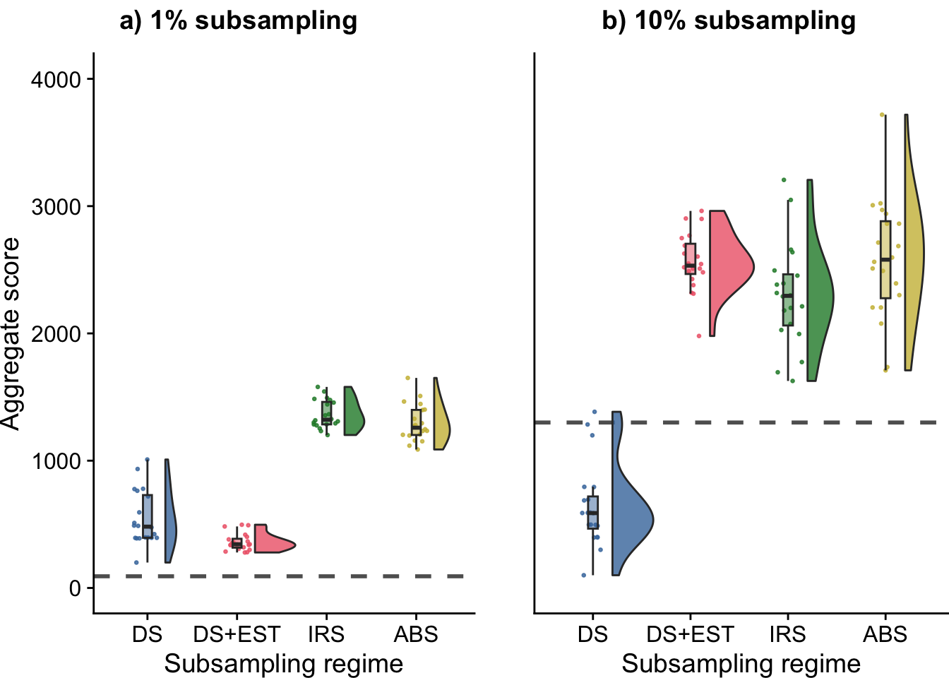

save_plot(
  filename = paste0(plot_directory, "2023-12-28-explore-lex-fig.pdf"),
  plot = lex_fig,
  base_width = 7,
  base_height = 3,
  dpi = 600
)