Chapter 7 Directed digital evolution experiment
Supplemental information and data analyses for the initial (baseline) directed evolution modeling experiment.
7.2 Analysis dependencies
Load all required R libraries
library(tidyverse)
library(ggplot2)
library(cowplot)
library(RColorBrewer)
library(khroma)
source("https://gist.githubusercontent.com/benmarwick/2a1bb0133ff568cbe28d/raw/fb53bd97121f7f9ce947837ef1a4c65a73bffb3f/geom_flat_violin.R")
These analyses were knit with the following environment:
##                _
## platform       x86_64-pc-linux-gnu
## arch           x86_64
## os             linux-gnu
## system         x86_64, linux-gnu
## status
## major          4
## minor          2.1
## year           2022
## month          06
## day            23
## svn rev        82513
## language       R
## version.string R version 4.2.1 (2022-06-23)
## nickname       Funny-Looking Kid
7.3 Setup
Load experiment summary data.
exp_summary_data_loc <- paste0(working_directory,"data/experiment_summary.csv")
exp_summary_data <- read.csv(exp_summary_data_loc, na.strings="NONE")

exp_summary_data$SELECTION_METHOD <- factor(
  exp_summary_data$SELECTION_METHOD,
  levels=c(
    "elite",
    "elite-10",
    "tournament",
    "lexicase",
    "non-dominated-elite",
    "random",
    "none"
  ),
  labels=c(
    "elite",
    "elite-10",
    "tourn",
    "lex",
    "nde",
    "random",
    "none"
  )
)
Load time series data.
times_series_data_loc <- paste0(working_directory,"data/evaluation_time_series_corrected.csv")
times_series_data <- read.csv(times_series_data_loc, na.strings="NONE")

# Specify experimental condition for each datum.
times_series_data$SELECTION_METHOD <- factor(
  times_series_data$SELECTION_METHOD,
  levels=c(
    "elite",
    "elite-10",
    "tournament",
    "lexicase",
    "non-dominated-elite",
    "non-dominated-tournament",
    "random",
    "none"
  ),
  labels=c(
    "elite",
    "elite-10",
    "tourn",
    "lex",
    "nde",
    "ndt",
    "random",
    "none"
  )
)

times_series_data$epoch_offset <- times_series_data$epoch+1
Load task coverage per population data.
task_coverage_per_pop_data_loc <- paste0(working_directory,"data/max_coverage_per_pop_cnt.csv")
task_coverage_per_pop_data <- read.csv(task_coverage_per_pop_data_loc, na.strings="NONE")

# Specify experimental condition for each datum.
task_coverage_per_pop_data$SELECTION_METHOD <- factor(
  task_coverage_per_pop_data$SELECTION_METHOD,
  levels=c(
    "elite",
    "elite-10",
    "tournament",
    "lexicase",
    "non-dominated-elite",
    "non-dominated-tournament",
    "random",
    "none"
  ),
  labels=c(
    "elite",
    "elite-10",
    "tourn",
    "lex",
    "nde",
    "ndt",
    "random",
    "none"
  )
)
Miscellaneous setup
# Configure our default graphing theme
theme_set(theme_cowplot())
# Palette
scale_fill_fun <- scale_fill_bright
scale_color_fun <- scale_color_bright
alpha <- 0.05
# Create a directory to store plots
plot_directory <- paste0(working_directory, "plots/")
dir.create(plot_directory, showWarnings=FALSE)

p_label <- function(p_value) {
  threshold = 0.0001
  if (p_value < threshold) {
    return(paste0("p < ", threshold))
  } else {
    return(paste0("p = ", p_value))
  }
}


selection_method_breaks <- c("elite", "elite-10", "tourn", "lex", "nde", "random", "none")
selection_method_labels <- c("ELITE", "TOP-10", "TOURN", "LEX", "NDE", "RAND", "NONE")
7.4 Best single-population task coverage
Best single-population task coverage at the end of the experiment.
max_trait_cov_fig <-
  ggplot(
    exp_summary_data,
    aes(
      x=SELECTION_METHOD,
      y=max_trait_coverage,
      fill=SELECTION_METHOD
    )
  ) +
  geom_flat_violin(
    position = position_nudge(x = .2, y = 0),
    alpha = .8,
    adjust=1.5
  ) +
  geom_point(
    mapping=aes(color=SELECTION_METHOD),
    position = position_jitter(height=0.1, width = .15),
    size = .5,
    alpha = 0.8
  ) +
  geom_boxplot(
    width = .1,
    outlier.shape = NA,
    alpha = 0.5
  ) +
  scale_y_continuous(
    name="Task Coverage",
    limits=c(-0.5,18.5),
    breaks=seq(0,18,2)
  ) +
  scale_x_discrete(
    name="Selection Method",
    breaks=selection_method_breaks,
    labels=selection_method_labels
  ) +
  scale_fill_fun() +
  scale_color_fun() +
  theme(
    legend.position="none"
  )

max_trait_cov_fig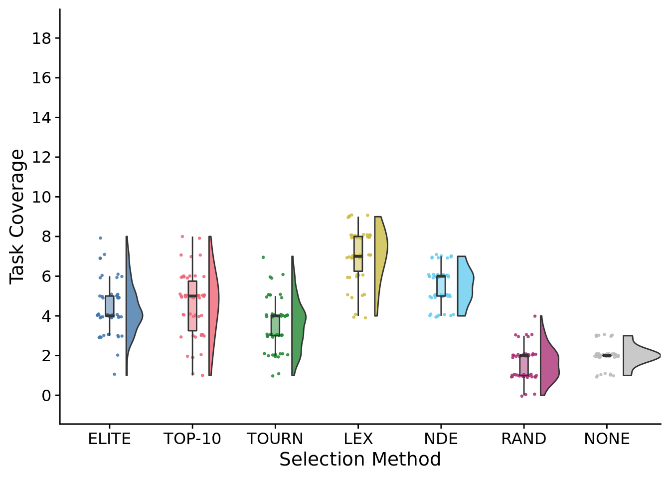
## Saving 7 x 5 in imageStatistical results:
##
##  Kruskal-Wallis rank sum test
##
## data:  max_trait_coverage by SELECTION_METHOD
## Kruskal-Wallis chi-squared = 244.55, df = 6, p-value < 2.2e-16
# Kruskal-wallis is significant, so we do a post-hoc wilcoxon rank-sum.
pairwise.wilcox.test(
x=exp_summary_data$max_trait_coverage,
g=exp_summary_data$SELECTION_METHOD,
p.adjust.method="bonferroni",
)##
## Pairwise comparisons using Wilcoxon rank sum test with continuity correction
##
## data: exp_summary_data$max_trait_coverage and exp_summary_data$SELECTION_METHOD
##
## elite elite-10 tourn lex nde random
## elite-10 1.0000 - - - - -
## tourn 0.0404 0.0167 - - - -
## lex 2.3e-11 9.6e-10 3.2e-14 - - -
## nde 0.0001 0.0234 6.8e-10 2.2e-07 - -
## random 1.2e-14 6.2e-13 1.7e-10 < 2e-16 < 2e-16 -
## none 1.0e-14 4.8e-12 1.1e-08 < 2e-16 < 2e-16 0.0392
##
## P value adjustment method: bonferroni7.4.1 Best single-population task coverage time series
To speed up graphing, we plot a low-resolution version of the time series.
max_trait_cov_ot_fig <-
  ggplot(
    # times_series_data,
    filter(times_series_data, (epoch_offset%%100)==0 | epoch_offset==1),
    aes(
      x=epoch_offset,
      y=max_trait_coverage,
      fill=SELECTION_METHOD,
      color=SELECTION_METHOD
    )
  ) +
  stat_summary(geom="line", fun=mean) +
  stat_summary(
    geom="ribbon",
    fun.data="mean_cl_boot",
    fun.args=list(conf.int=0.95),
    alpha=0.2,
    linetype=0
  ) +
  scale_x_continuous(
    name="Cycles"
  ) +
  scale_y_continuous(
    name="Task Coverage",
    limits=c(-0.5,18.5),
    breaks=seq(0,18,2)
  ) +
  scale_fill_fun(
    name="Selection Method",
    breaks=selection_method_breaks,
    labels=selection_method_labels
  ) +
  scale_color_fun(
    name="Selection Method",
    breaks=selection_method_breaks,
    labels=selection_method_labels
  ) +
  theme(
    legend.position="none"
  )
max_trait_cov_ot_fig
## Warning: Computation failed in `stat_summary()`: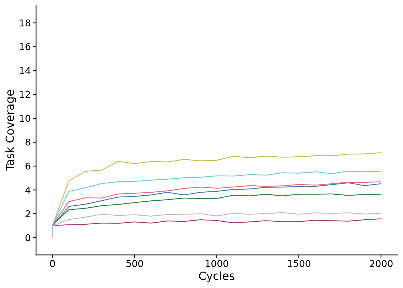
ggsave(
  plot=max_trait_cov_ot_fig,
  filename=paste0(plot_directory, "2021-11-11-best-pop-task-cov-ts.pdf"),
  width=10,
  height=6
)
## Warning: Computation failed in `stat_summary()`:7.4.1.1 First 30 cycles of the experiment
max_trait_cov_ot_early_fig <-
  ggplot(
    # times_series_data,
    filter(times_series_data, (epoch_offset <= 30)),
    aes(
      x=epoch_offset,
      y=max_trait_coverage,
      fill=SELECTION_METHOD,
      color=SELECTION_METHOD
    )
  ) +
  stat_summary(geom="line", fun=mean) +
  stat_summary(
    geom="ribbon",
    fun.data="mean_cl_boot",
    fun.args=list(conf.int=0.95),
    alpha=0.2,
    linetype=0
  ) +
  scale_x_continuous(
    name="Cycles"
  ) +
  scale_y_continuous(
    name="Task Coverage",
    limits=c(-0.5,18.5),
    breaks=seq(0,18,2)
  ) +
  scale_fill_fun(
    name="Selection Method",

    breaks=selection_method_breaks,
    labels=selection_method_labels
  ) +
  scale_color_fun(
    name="Selection Method",

    breaks=selection_method_breaks,
    labels=selection_method_labels
  ) +
  theme(
    legend.position="bottom"
  )
max_trait_cov_ot_early_fig
## Warning: Computation failed in `stat_summary()`: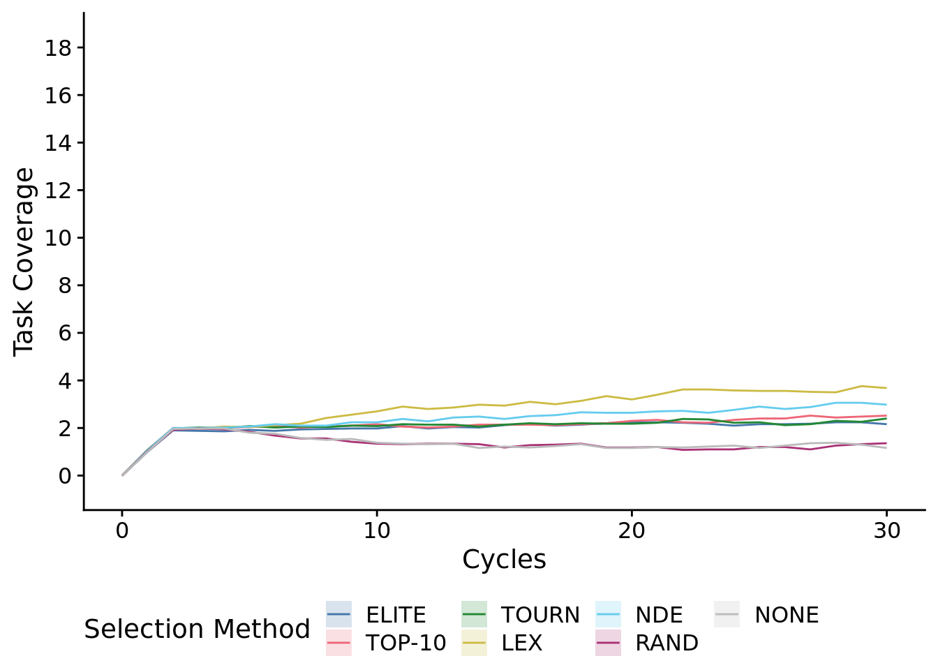
ggsave(
  filename=paste0(plot_directory, "2021-11-11-best-pop-task-cov-ts-early.pdf"),
  width=10,
  height=6
)
## Warning: Computation failed in `stat_summary()`:After just 10 cycles, we observed significant gains from using NDE and LEX selection protocols.
early_data <- filter(times_series_data, epoch_offset==10)
kruskal.test(
  formula=max_trait_coverage~SELECTION_METHOD,
  data=early_data
)
##
## Kruskal-Wallis rank sum test
##
## data: max_trait_coverage by SELECTION_METHOD
## Kruskal-Wallis chi-squared = 166.2, df = 6, p-value < 2.2e-16# Kruskal-wallis is significant, so we do a post-hoc wilcoxon rank-sum.
pairwise.wilcox.test(
x=early_data$max_trait_coverage,
g=early_data$SELECTION_METHOD,
p.adjust.method="bonferroni",
)##
## Pairwise comparisons using Wilcoxon rank sum test with continuity correction
##
## data: early_data$max_trait_coverage and early_data$SELECTION_METHOD
##
## elite elite-10 tourn lex nde random
## elite-10 1.00000 - - - - -
## tourn 1.00000 1.00000 - - - -
## lex 2.1e-06 0.00087 2.3e-06 - - -
## nde 0.14106 1.00000 0.63684 0.00709 - -
## random 3.3e-07 5.5e-10 5.2e-11 1.2e-13 1.7e-11 -
## none 2.0e-06 3.2e-09 3.9e-10 3.6e-13 9.5e-11 1.00000
##
## P value adjustment method: bonferroni7.5 Metapopulation task coverage
Metapopulation task coverage at the end of the experiment.
total_trait_cov_fig <-
  ggplot(
    exp_summary_data,
    aes(
      x=SELECTION_METHOD,
      y=total_trait_coverage,
      fill=SELECTION_METHOD
    )
  ) +
  geom_flat_violin(
    position = position_nudge(x = .2, y = 0),
    alpha = .8,
    adjust=1.5
  ) +
  geom_point(
    mapping=aes(color=SELECTION_METHOD),
    position = position_jitter(height=0.1, width = .15),
    size = .5,
    alpha = 0.8
  ) +
  geom_boxplot(
    width = .1,
    outlier.shape = NA,
    alpha = 0.5
  ) +
  scale_y_continuous(
    name="Task Coverage",
    limits=c(-0.5,18.5),
    breaks=seq(0,18,2)
  ) +
  scale_x_discrete(
    name="Selection Method",
    breaks=selection_method_breaks,
    labels=selection_method_labels
  ) +
  scale_fill_fun(
  ) +
  scale_color_fun(
  ) +
  theme(
    legend.position="none"
  )

total_trait_cov_fig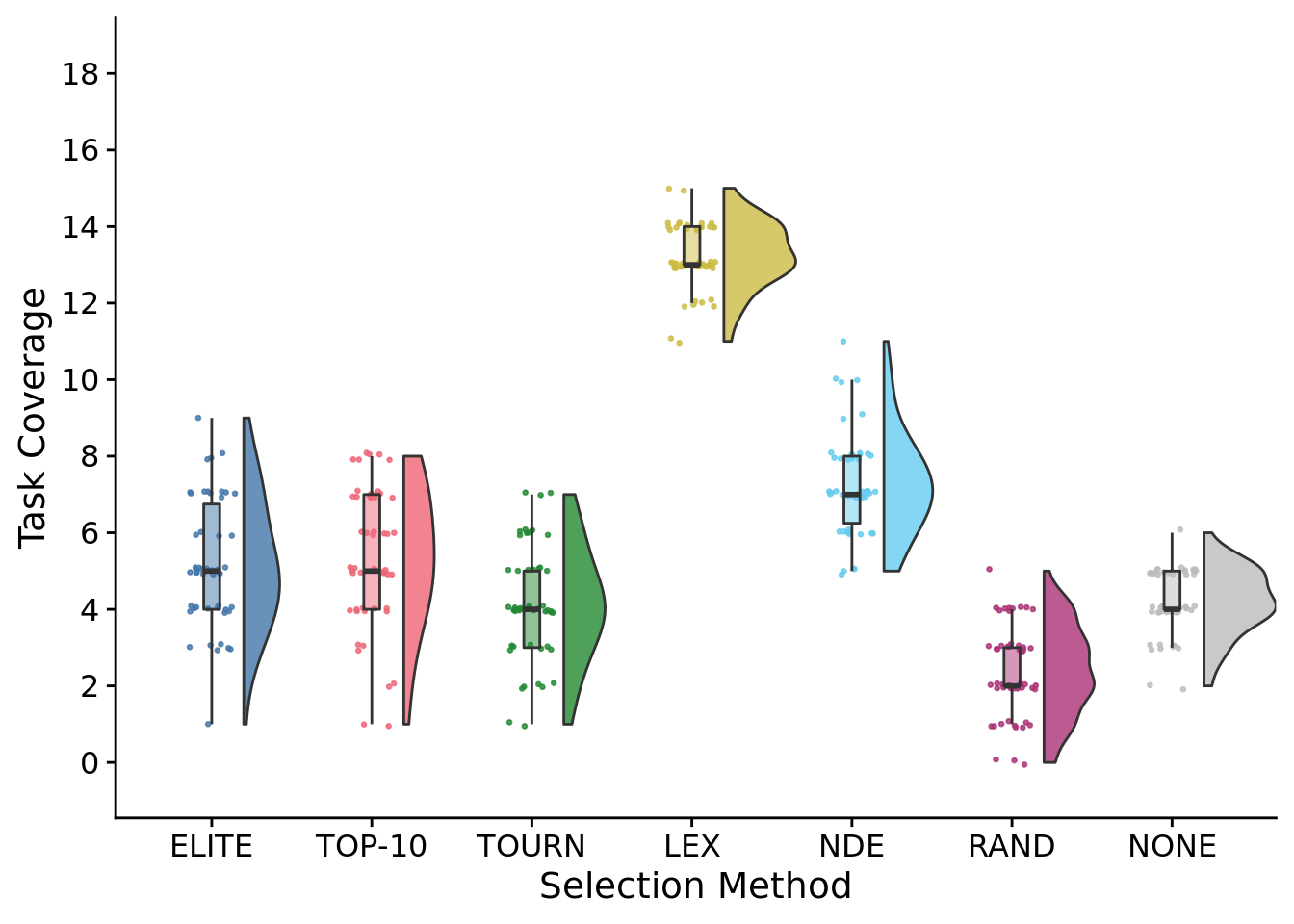
## Saving 7 x 5 in imageStatistical results:
##
##  Kruskal-Wallis rank sum test
##
## data:  total_trait_coverage by SELECTION_METHOD
## Kruskal-Wallis chi-squared = 244.66, df = 6, p-value < 2.2e-16
# Kruskal-wallis is significant, so we do a post-hoc wilcoxon rank-sum.
pairwise.wilcox.test(
x=exp_summary_data$total_trait_coverage,
g=exp_summary_data$SELECTION_METHOD,
p.adjust.method="bonferroni",
)##
## Pairwise comparisons using Wilcoxon rank sum test with continuity correction
##
## data: exp_summary_data$total_trait_coverage and exp_summary_data$SELECTION_METHOD
##
## elite elite-10 tourn lex nde random
## elite-10 1.0000 - - - - -
## tourn 0.0513 0.0079 - - - -
## lex < 2e-16 < 2e-16 < 2e-16 - - -
## nde 1.5e-07 1.1e-05 2.1e-13 < 2e-16 - -
## random 8.3e-12 5.9e-11 6.1e-07 < 2e-16 < 2e-16 -
## none 0.0261 0.0017 1.0000 < 2e-16 6.7e-16 5.4e-10
##
## P value adjustment method: bonferroni7.5.1 Metapopulation task coverage time series
To speed up plotting, we graph a low-resolution version of this time series.
metapop_task_cov_ot_fig <-
  ggplot(
    # times_series_data,
    filter(times_series_data, (epoch_offset%%100)==0 | epoch_offset==1),
    aes(
      x=epoch_offset,
      y=total_trait_coverage,
      fill=SELECTION_METHOD,
      color=SELECTION_METHOD
    )
  ) +
  stat_summary(geom="line", fun=mean) +
  stat_summary(
    geom="ribbon",
    fun.data="mean_cl_boot",
    fun.args=list(conf.int=0.95),
    alpha=0.2,
    linetype=0
  ) +
    scale_x_continuous(
    name="Cycles"
  ) +
  scale_y_continuous(
    name="Task Coverage",
    limits=c(-0.5,18.5),
    breaks=seq(0,18,2)
  ) +
  scale_fill_fun(
    name="Selection Method",
    breaks=selection_method_breaks,
    labels=selection_method_labels
  ) +
  scale_color_fun(
    name="Selection Method",
    breaks=selection_method_breaks,
    labels=selection_method_labels
  ) +
  theme(
    legend.position="bottom"
  )
metapop_task_cov_ot_fig
## Warning: Computation failed in `stat_summary()`: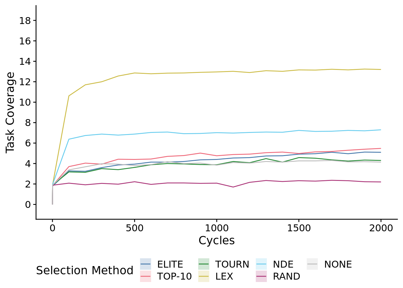
ggsave(
  plot=metapop_task_cov_ot_fig,
  filename=paste0(plot_directory, "2021-11-11-metapop-task-cov-ts.pdf"),
  width=10,
  height=6
)
## Warning: Computation failed in `stat_summary()`:7.5.1.1 First 30 cycles of the experiment
metapop_task_cov_ot_early_fig <-
  ggplot(
    # times_series_data,
    filter(times_series_data, (epoch_offset <= 30)),
    aes(
      x=epoch_offset,
      y=total_trait_coverage,
      fill=SELECTION_METHOD,
      color=SELECTION_METHOD
    )
  ) +
  stat_summary(geom="line", fun=mean) +
  stat_summary(
    geom="ribbon",
    fun.data="mean_cl_boot",
    fun.args=list(conf.int=0.95),
    alpha=0.2,
    linetype=0
  ) +
  scale_x_continuous(
    name="Cycles"
  ) +
  scale_y_continuous(
    name="Task Coverage",
    limits=c(-0.5,18.5),
    breaks=seq(0,18,2)
  ) +
  scale_fill_fun(
    name="Selection Method",
    breaks=selection_method_breaks,
    labels=selection_method_labels
  ) +
  scale_color_fun(
    name="Selection Method",
    breaks=selection_method_breaks,
    labels=selection_method_labels
  ) +
  theme(
    legend.position="bottom"
  )
metapop_task_cov_ot_early_fig
## Warning: Computation failed in `stat_summary()`: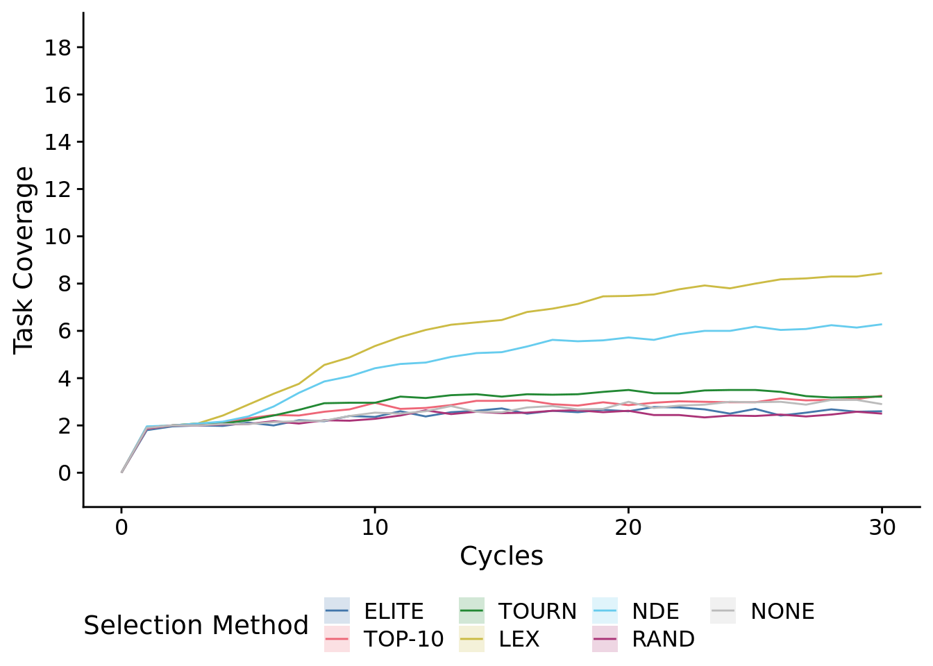
ggsave(
  filename=paste0(plot_directory, "2021-11-11-metapop-task-cov-ts-early.pdf"),
  width=10,
  height=6
)
## Warning: Computation failed in `stat_summary()`:After just 10 cycles, we observed significant gains from using NDE and LEX selection protocols.
early_data <- filter(times_series_data, epoch_offset==10)
kruskal.test(
  formula=total_trait_coverage~SELECTION_METHOD,
  data=early_data
)
##
## Kruskal-Wallis rank sum test
##
## data: total_trait_coverage by SELECTION_METHOD
## Kruskal-Wallis chi-squared = 180.78, df = 6, p-value < 2.2e-16# Kruskal-wallis is significant, so we do a post-hoc wilcoxon rank-sum.
pairwise.wilcox.test(
x=early_data$total_trait_coverage,
g=early_data$SELECTION_METHOD,
p.adjust.method="bonferroni",
)##
## Pairwise comparisons using Wilcoxon rank sum test with continuity correction
##
## data: early_data$total_trait_coverage and early_data$SELECTION_METHOD
##
## elite elite-10 tourn lex nde random
## elite-10 0.06728 - - - - -
## tourn 0.01593 1.00000 - - - -
## lex 3.7e-14 9.8e-11 1.3e-11 - - -
## nde 1.7e-12 1.9e-07 1.8e-08 0.03737 - -
## random 1.00000 0.00627 0.00051 7.7e-16 4.9e-15 -
## none 1.00000 0.93717 0.28402 8.7e-15 2.6e-13 0.38944
##
## P value adjustment method: bonferroni7.6 Metapopulation task profile diversity
We measured the “phenotypic” diversity within evolved metapopulations in three ways:
- the number of task profiles (richness)
- the spread of task profiles as the average cosine distance from the centroid profile
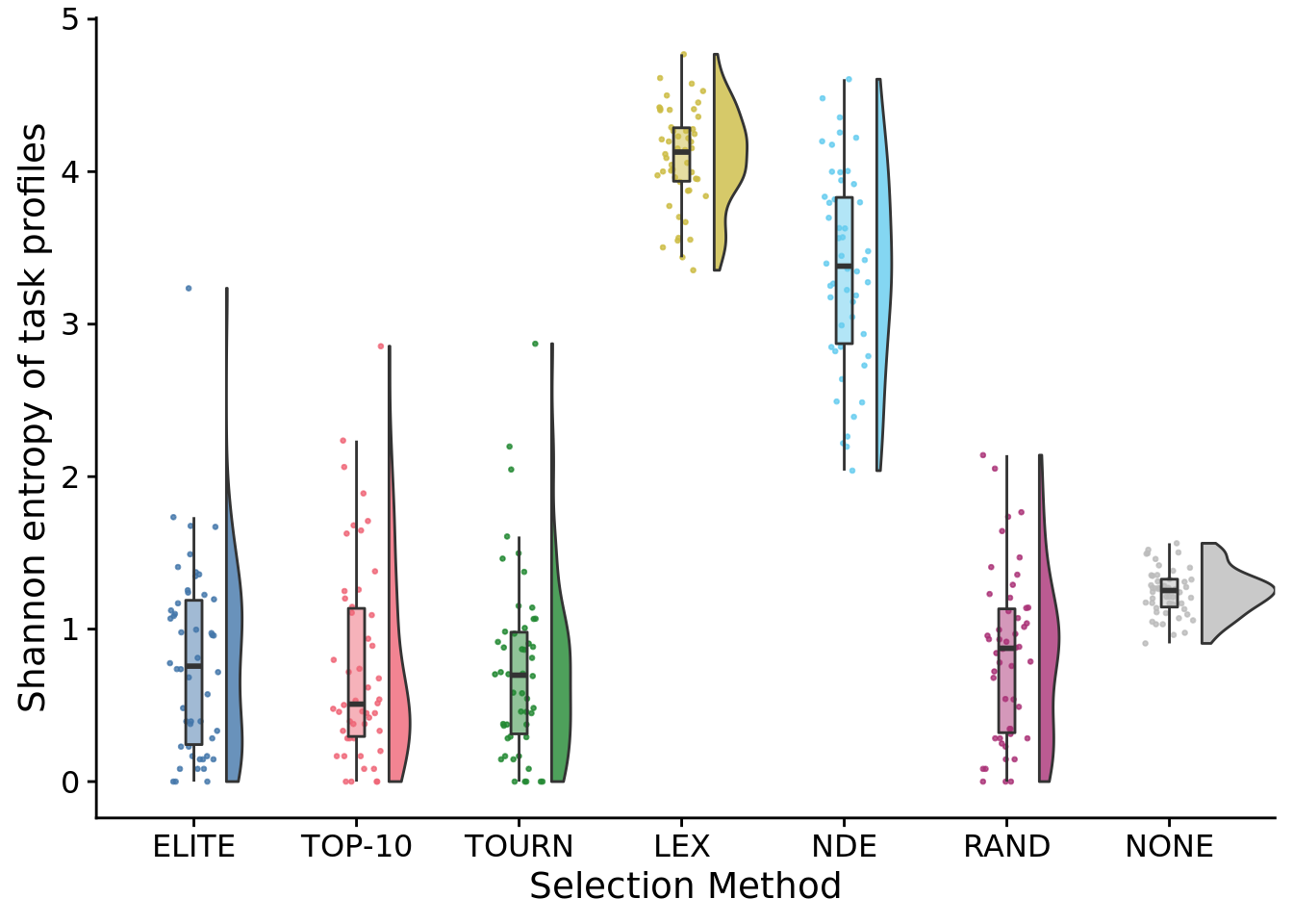
- the Shannon entropy of task profiles
7.6.1 Number of different task profiles
num_pop_task_profiles_fig <-
  ggplot(
    exp_summary_data,
    aes(
      x=SELECTION_METHOD,
      y=num_pop_trait_profiles,
      fill=SELECTION_METHOD
    )
  ) +
  geom_flat_violin(
    position = position_nudge(x = .2, y = 0),
    alpha = .8
  ) +
  geom_point(
    mapping=aes(color=SELECTION_METHOD),
    position = position_jitter(height=0, width = .15),
    size = .5,
    alpha = 0.8
  ) +
  geom_boxplot(
    width = .1,
    outlier.shape = NA,
    alpha = 0.5
  ) +
  scale_y_continuous(
    name="# Different Task Profiles"
  ) +
  scale_x_discrete(
    name="Selection Method",
    breaks=selection_method_breaks,
    labels=selection_method_labels
  ) +
  scale_fill_fun(
  ) +
  scale_color_fun(
  ) +
  theme(
    legend.position="none"
  )
num_pop_task_profiles_fig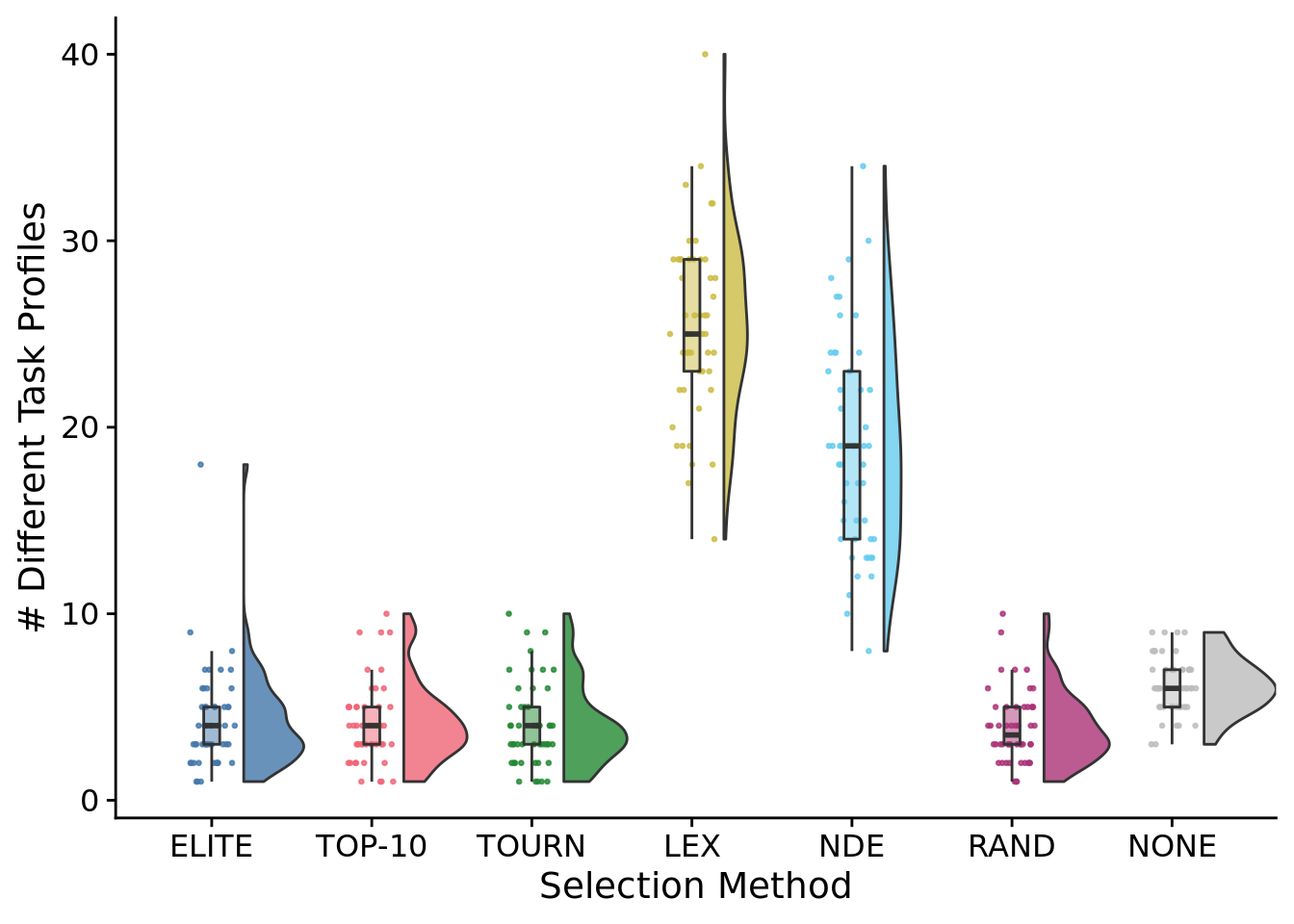
ggsave(
  plot=num_pop_task_profiles_fig,
  paste0(plot_directory, "2021-11-11-num-task-profiles.pdf")
)
## Saving 7 x 5 in imageStatistical results:
##
##  Kruskal-Wallis rank sum test
##
## data:  num_pop_trait_profiles by SELECTION_METHOD
## Kruskal-Wallis chi-squared = 239.62, df = 6, p-value < 2.2e-16
# Kruskal-wallis is significant, so we do a post-hoc wilcoxon rank-sum.
pairwise.wilcox.test(
x=exp_summary_data$num_pop_trait_profiles,
g=exp_summary_data$SELECTION_METHOD,
p.adjust.method="bonferroni",
)##
## Pairwise comparisons using Wilcoxon rank sum test with continuity correction
##
## data: exp_summary_data$num_pop_trait_profiles and exp_summary_data$SELECTION_METHOD
##
## elite elite-10 tourn lex nde random
## elite-10 1 - - - - -
## tourn 1 1 - - - -
## lex < 2e-16 < 2e-16 < 2e-16 - - -
## nde 5.3e-16 < 2e-16 < 2e-16 3.2e-06 - -
## random 1 1 1 < 2e-16 < 2e-16 -
## none 6.2e-06 2.2e-06 5.1e-06 < 2e-16 < 2e-16 1.5e-07
##
## P value adjustment method: bonferroni7.6.1.1 Number of different task profiles over time
num_task_profiles_ot_fig <-
  ggplot(
    filter(times_series_data, (updates_elapsed%%10000)==0 | updates_elapsed==1),
    aes(
      x=updates_elapsed,
      y=num_pop_trait_profiles,
      fill=SELECTION_METHOD,
      color=SELECTION_METHOD
    )
  ) +
  stat_summary(geom="line", fun=mean) +
  stat_summary(
    geom="ribbon",
    fun.data="mean_cl_boot",
    fun.args=list(conf.int=0.95),
    alpha=0.2,
    linetype=0
  ) +
  scale_x_continuous(
    name="Updates elapsed"
  ) +
  scale_y_continuous(
    name="# Different Task Profiles"
  ) +
  scale_fill_fun(
    name="Selection Method",
    breaks=selection_method_breaks,
    labels=selection_method_labels
  ) +
  scale_color_fun(
    name="Selection Method",
    breaks=selection_method_breaks,
    labels=selection_method_labels
  ) +
  theme(
    legend.position="bottom"
  )
num_task_profiles_ot_fig
## Warning: Computation failed in `stat_summary()`: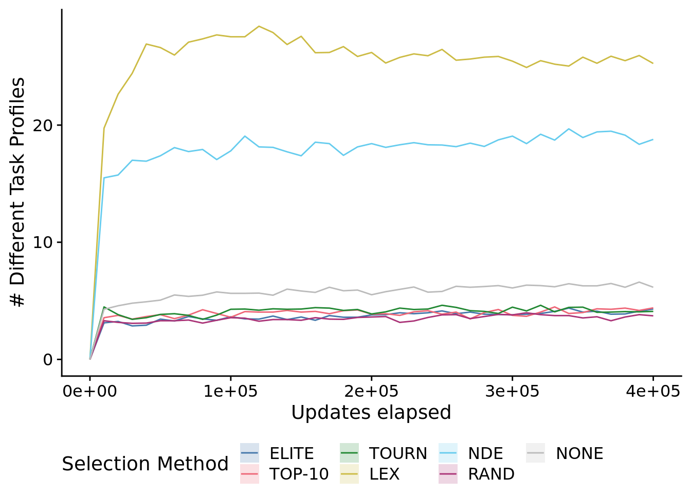
ggsave(
  num_task_profiles_ot_fig,
  filename=paste0(plot_directory, "2021-11-11-num-task-profiles-ts.png"),
  width=10,
  height=6
)
## Warning: Computation failed in `stat_summary()`:7.6.2 Task profile spread
task_profile_spread_fig <-
  ggplot(
    exp_summary_data,
    aes(
      x=SELECTION_METHOD,
      y=avg_cosine_dist_from_centroid,
      fill=SELECTION_METHOD
    )
  ) +
  geom_flat_violin(
    position = position_nudge(x = .2, y = 0),
    alpha = .8
  ) +
  geom_point(
    mapping=aes(color=SELECTION_METHOD),
    position = position_jitter(height=0, width = .15),
    size = .5,
    alpha = 0.8
  ) +
  geom_boxplot(
    width = .1,
    outlier.shape = NA,
    alpha = 0.5
  ) +
  scale_y_continuous(
    name="Avg. Task Spread"
  ) +
  scale_x_discrete(
    name="Selection Method",
    breaks=selection_method_breaks,
    labels=selection_method_labels
  ) +
  scale_fill_fun(
  ) +
  scale_color_fun(
  ) +
  theme(
    legend.position="none"
  )
task_profile_spread_fig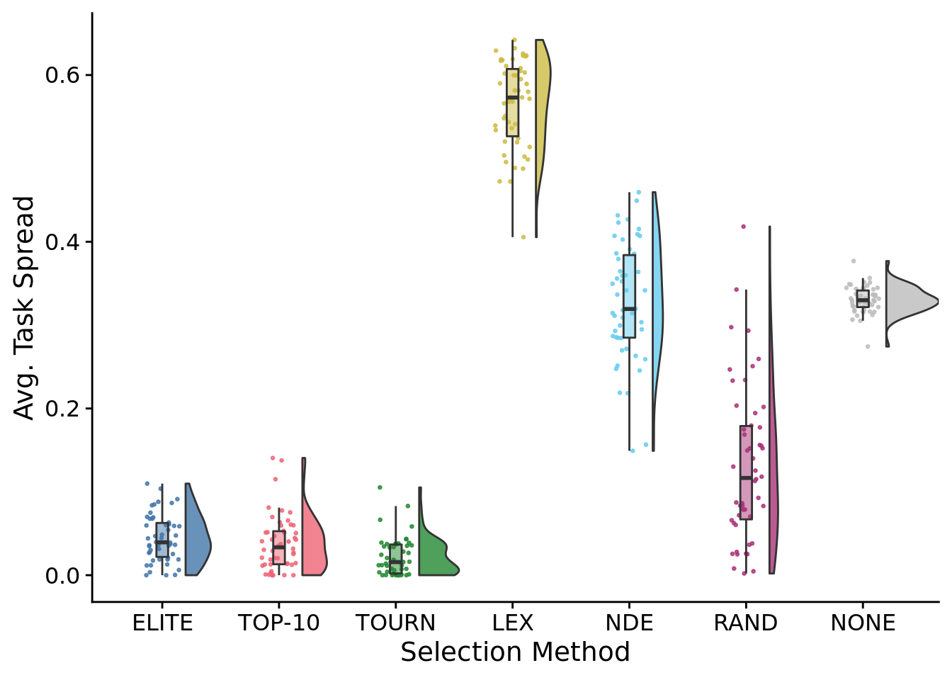
ggsave(
  plot=task_profile_spread_fig,
  paste0(plot_directory, "2021-11-11-task-profile-spread.pdf")
)
## Saving 7 x 5 in imageStatistical results:
##
##  Kruskal-Wallis rank sum test
##
## data:  avg_cosine_dist_from_centroid by SELECTION_METHOD
## Kruskal-Wallis chi-squared = 292.39, df = 6, p-value < 2.2e-16
# Kruskal-wallis is significant, so we do a post-hoc wilcoxon rank-sum.
pairwise.wilcox.test(
x=exp_summary_data$avg_cosine_dist_from_centroid,
g=exp_summary_data$SELECTION_METHOD,
p.adjust.method="bonferroni",
)##
## Pairwise comparisons using Wilcoxon rank sum test with continuity correction
##
## data: exp_summary_data$avg_cosine_dist_from_centroid and exp_summary_data$SELECTION_METHOD
##
## elite elite-10 tourn lex nde random
## elite-10 1.00000 - - - - -
## tourn 0.00069 0.13725 - - - -
## lex < 2e-16 < 2e-16 < 2e-16 - - -
## nde < 2e-16 < 2e-16 < 2e-16 2.5e-16 - -
## random 1.8e-06 7.7e-08 1.0e-10 < 2e-16 8.5e-13 -
## none < 2e-16 < 2e-16 < 2e-16 < 2e-16 1.00000 2.6e-14
##
## P value adjustment method: bonferroni7.6.3 Task profile entropy
ggplot(
    exp_summary_data,
    aes(
      x=SELECTION_METHOD,
      y=pop_trait_profile_entropy,
      fill=SELECTION_METHOD
    )
  ) +
  geom_flat_violin(
    position = position_nudge(x = .2, y = 0),
    alpha = .8
  ) +
  geom_point(
    mapping=aes(color=SELECTION_METHOD),
    position = position_jitter(height=0, width = .15),
    size = .5,
    alpha = 0.8
  ) +
  geom_boxplot(
    width = .1,
    outlier.shape = NA,
    alpha = 0.5
  ) +
  scale_y_continuous(
    name="Shannon entropy of task profiles"
  ) +
  scale_x_discrete(
    name="Selection Method",
    breaks=selection_method_breaks,
    labels=selection_method_labels
  ) +
  scale_fill_fun(
  ) +
  scale_color_fun(
  ) +
  theme(
    legend.position="none"
  )
## Saving 7 x 5 in imageStatistical results:
##
##  Kruskal-Wallis rank sum test
##
## data:  pop_trait_profile_entropy by SELECTION_METHOD
## Kruskal-Wallis chi-squared = 237.28, df = 6, p-value < 2.2e-16pairwise.wilcox.test(
x=exp_summary_data$pop_trait_profile_entropy,
g=exp_summary_data$SELECTION_METHOD,
p.adjust.method="bonferroni",
)##
## Pairwise comparisons using Wilcoxon rank sum test with continuity correction
##
## data: exp_summary_data$pop_trait_profile_entropy and exp_summary_data$SELECTION_METHOD
##
## elite elite-10 tourn lex nde random
## elite-10 1 - - - - -
## tourn 1 1 - - - -
## lex < 2e-16 < 2e-16 < 2e-16 - - -
## nde 4.9e-16 4.1e-16 3.8e-16 1.3e-07 - -
## random 1 1 1 < 2e-16 < 2e-16 -
## none 3.9e-05 2.2e-05 4.7e-08 < 2e-16 < 2e-16 9.1e-06
##
## P value adjustment method: bonferroni7.6.3.1 Task entropy over time
ggplot(
    filter(times_series_data, (updates_elapsed%%10000)==0 | updates_elapsed==1),
    aes(
      x=updates_elapsed,
      y=pop_trait_profile_entropy,
      fill=SELECTION_METHOD,
      color=SELECTION_METHOD
    )
  ) +
  stat_summary(geom="line", fun=mean) +
  stat_summary(
    geom="ribbon",
    fun.data="mean_cl_boot",
    fun.args=list(conf.int=0.95),
    alpha=0.2,
    linetype=0
  ) +
  scale_x_continuous(
    name="Updates elapsed"
  ) +
  scale_y_continuous(
    name="Task profile entropy"
  ) +
  scale_fill_fun(
    name="Selection Method",
    breaks=selection_method_breaks,
    labels=selection_method_labels
  ) +
  scale_color_fun(
    name="Selection Method",
    breaks=selection_method_breaks,
    labels=selection_method_labels
  ) +
  theme(
    legend.position="bottom"
  )
## Warning: Computation failed in `stat_summary()`: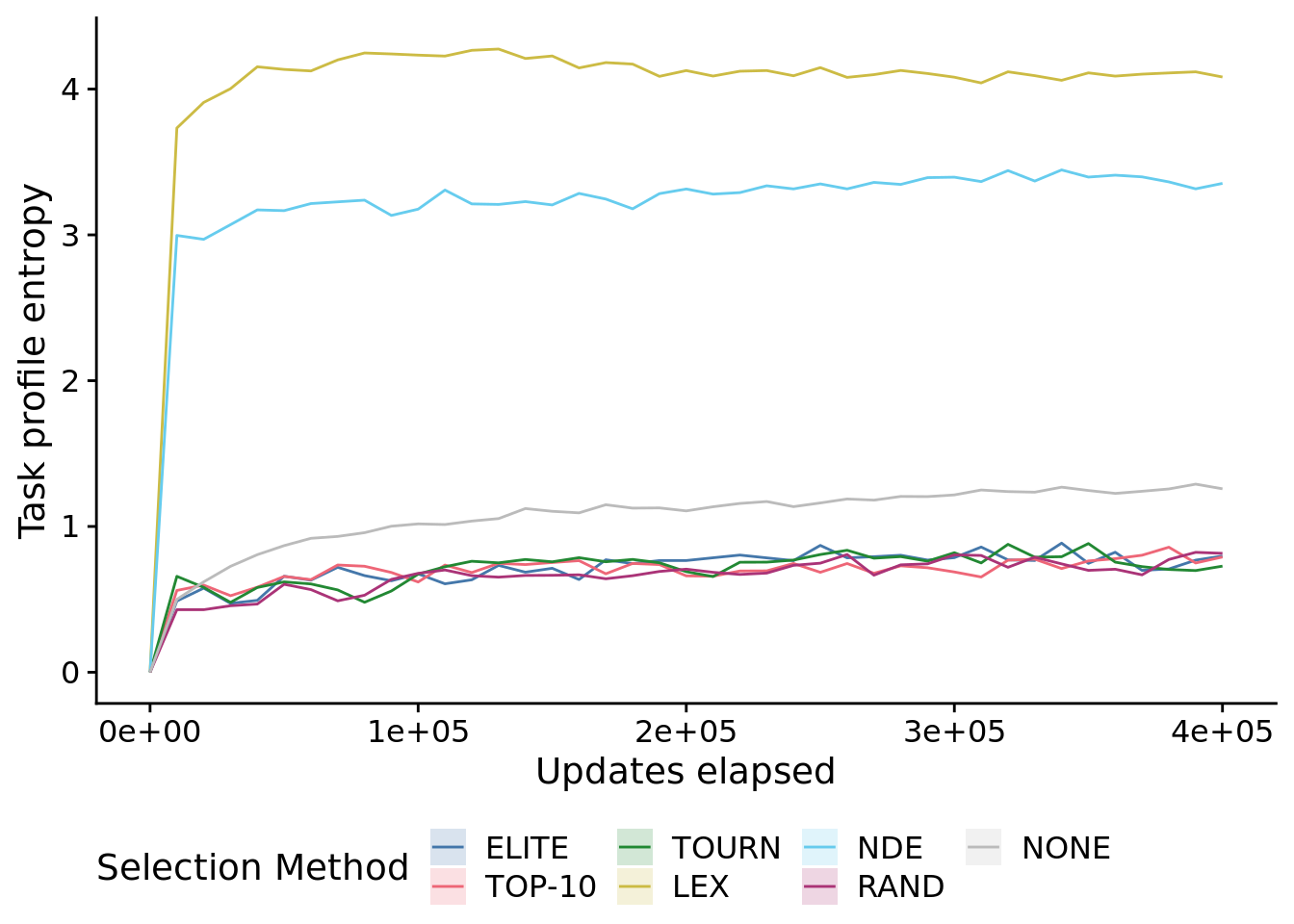
ggsave(
  filename=paste0(plot_directory, "2021-11-11-pop-trait-profile-entropy-ts.png"),
  width=10,
  height=6
)
## Warning: Computation failed in `stat_summary()`:7.7 Task coverage per N populations
We analyzed the (maximum) number of tasks added to metapopulation task coverage for a given number (N) of member populations considered. That is, for each N, we solved the maximum set coverage problem for task coverage: what is the maximum number of tasks that can be covered given N populations from this metapopulation?
ggplot(
    task_coverage_per_pop_data,
    aes(
      x=n_pops,
      y=max_tasks_covered,
      fill=SELECTION_METHOD,
      color=SELECTION_METHOD
    )
  ) +
  stat_summary(geom="line", fun=mean) +
  stat_summary(
    geom="ribbon",
    fun.data="mean_cl_boot",
    fun.args=list(conf.int=0.95),
    alpha=0.2,
    linetype=0
  ) +
  scale_y_continuous(
    name="Maximum task coverage"
  ) +
  scale_x_continuous(
    name="Number of populations",
    limits=c(0, 15)
  ) +
  scale_fill_fun(
    name="Selection Method",
    breaks=selection_method_breaks,
    labels=selection_method_labels
  ) +
  scale_color_fun(
    name="Selection Method",
    breaks=selection_method_breaks,
    labels=selection_method_labels
  ) +
  theme(
    legend.position="bottom"
  )
## Warning: Removed 28350 rows containing non-finite values (stat_summary).
## Removed 28350 rows containing non-finite values (stat_summary).## Warning: Computation failed in `stat_summary()`: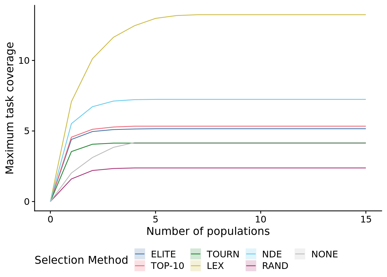
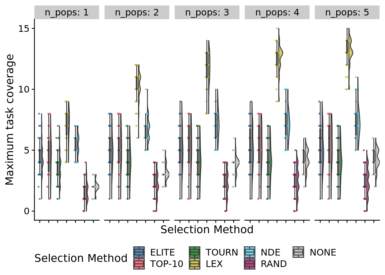
## Warning: Removed 28350 rows containing non-finite values (stat_summary).## Warning: Removed 28350 rows containing non-finite values (stat_summary).## Warning: Computation failed in `stat_summary()`:ggplot(
filter(
task_coverage_per_pop_data,
n_pops > 0 & n_pops <= 5
),
aes(
x=SELECTION_METHOD,
y=max_tasks_covered,
fill=SELECTION_METHOD
)
) +
geom_flat_violin(
position = position_nudge(x = .2, y = 0),
alpha = .8
) +
geom_point(
mapping=aes(color=SELECTION_METHOD),
position = position_jitter(height=0, width = .15),
size = .5,
alpha = 0.8
) +
geom_boxplot(
width = .1,
outlier.shape = NA,
alpha = 0.5
) +
scale_y_continuous(
name="Maximum task coverage"
) +
scale_x_discrete(
name="Selection Method",
breaks=selection_method_breaks,
labels=selection_method_labels
) +
scale_fill_fun(
name="Selection Method",
breaks=selection_method_breaks,
labels=selection_method_labels
) +
scale_color_fun(
name="Selection Method",
breaks=selection_method_breaks,
labels=selection_method_labels
) +
facet_wrap(
~n_pops,
nrow=1,
labeller=label_both
) +
theme(
legend.position="bottom",
axis.text.x = element_blank()
)
7.8 Average number of different populations selected per generation
ggplot(
    exp_summary_data,
    aes(
      x=SELECTION_METHOD,
      y=avg_unique_selected,
      fill=SELECTION_METHOD
    )
  ) +
  geom_flat_violin(
    position = position_nudge(x = .2, y = 0),
    alpha = .8
  ) +
  geom_point(
    mapping=aes(color=SELECTION_METHOD),
    position = position_jitter(height=0, width = .15),
    size = .5,
    alpha = 0.8
  ) +
  geom_boxplot(
    width = .1,
    outlier.shape = NA,
    alpha = 0.5
  ) +
  scale_y_continuous(
    name="Avg. number selected"
  ) +
  scale_x_discrete(
    name="Selection Method",
    breaks=selection_method_breaks,
    labels=selection_method_labels
  ) +
  scale_fill_fun(
    name="Selection Method",
    breaks=selection_method_breaks,
    labels=selection_method_labels
  ) +
  scale_color_fun(
    name="Selection Method",
    breaks=selection_method_breaks,
    labels=selection_method_labels
  ) +
  theme(
    legend.position="none"
  )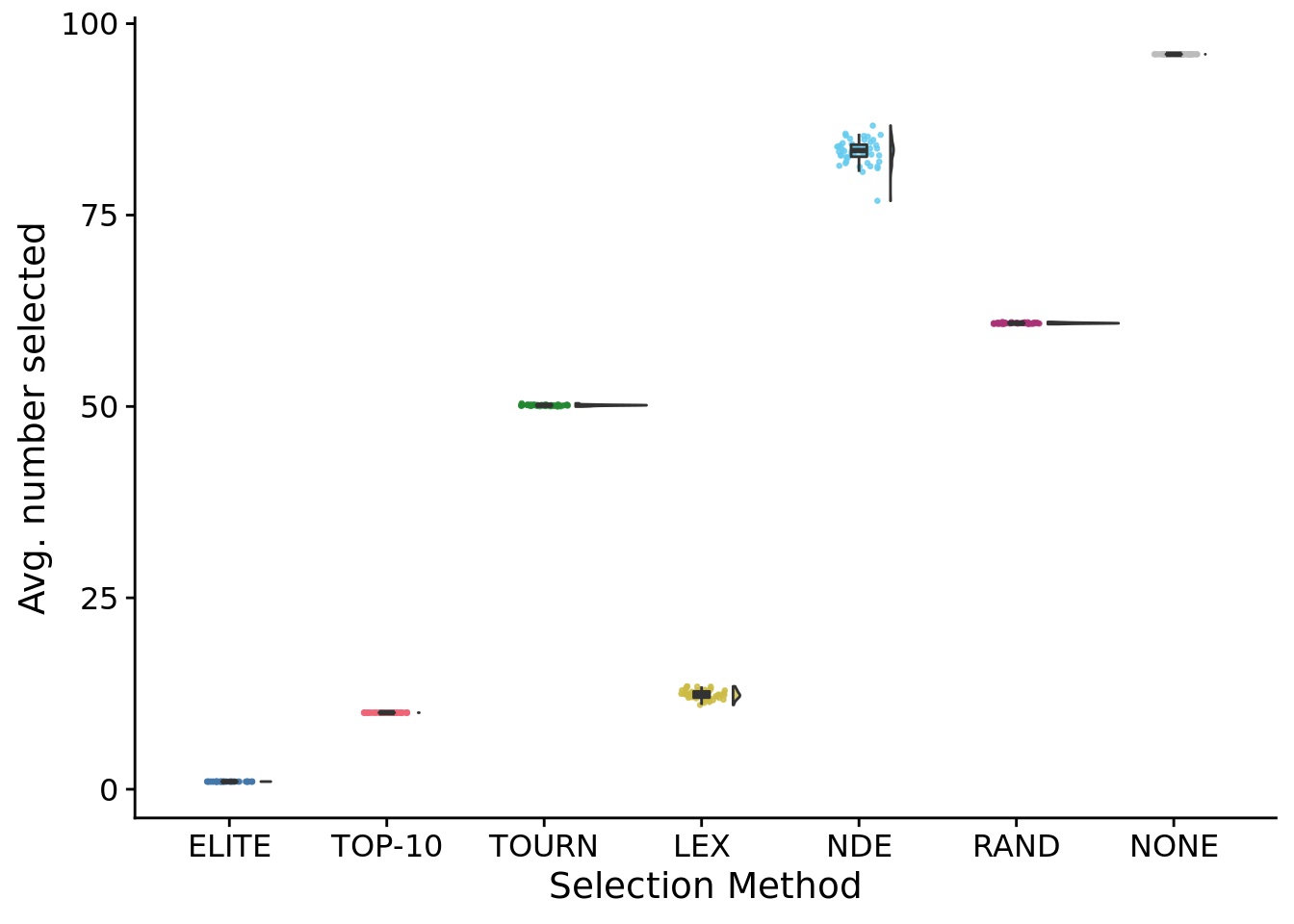
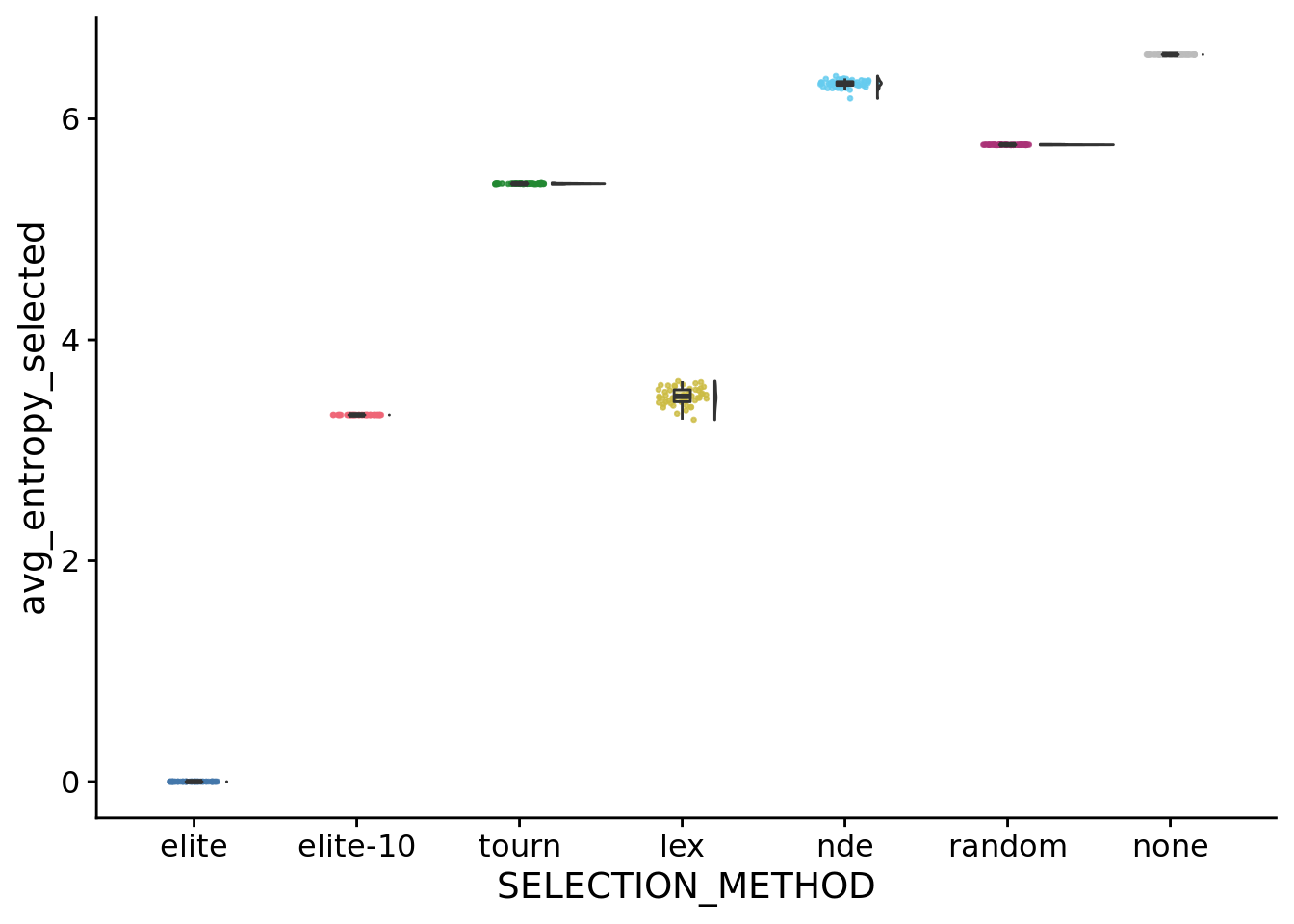
## Saving 7 x 5 in image## [1] 1## [1] 10## [1] 50.14939## [1] 83.29294## [1] 12.36869## [1] 60.877757.8.1 Entropy of selected population IDs
ggplot(
    exp_summary_data,
    aes(
      x=SELECTION_METHOD,
      y=avg_entropy_selected,
      fill=SELECTION_METHOD
    )
  ) +
  geom_flat_violin(
    position = position_nudge(x = .2, y = 0),
    alpha = .8
  ) +
  geom_point(
    mapping=aes(color=SELECTION_METHOD),
    position = position_jitter(height=0, width = .15),
    size = .5,
    alpha = 0.8
  ) +
  geom_boxplot(
    width = .1,
    outlier.shape = NA,
    alpha = 0.5
  ) +
  scale_fill_fun(
  ) +
  scale_color_fun(
  ) +
  theme(
    legend.position="none"
  )
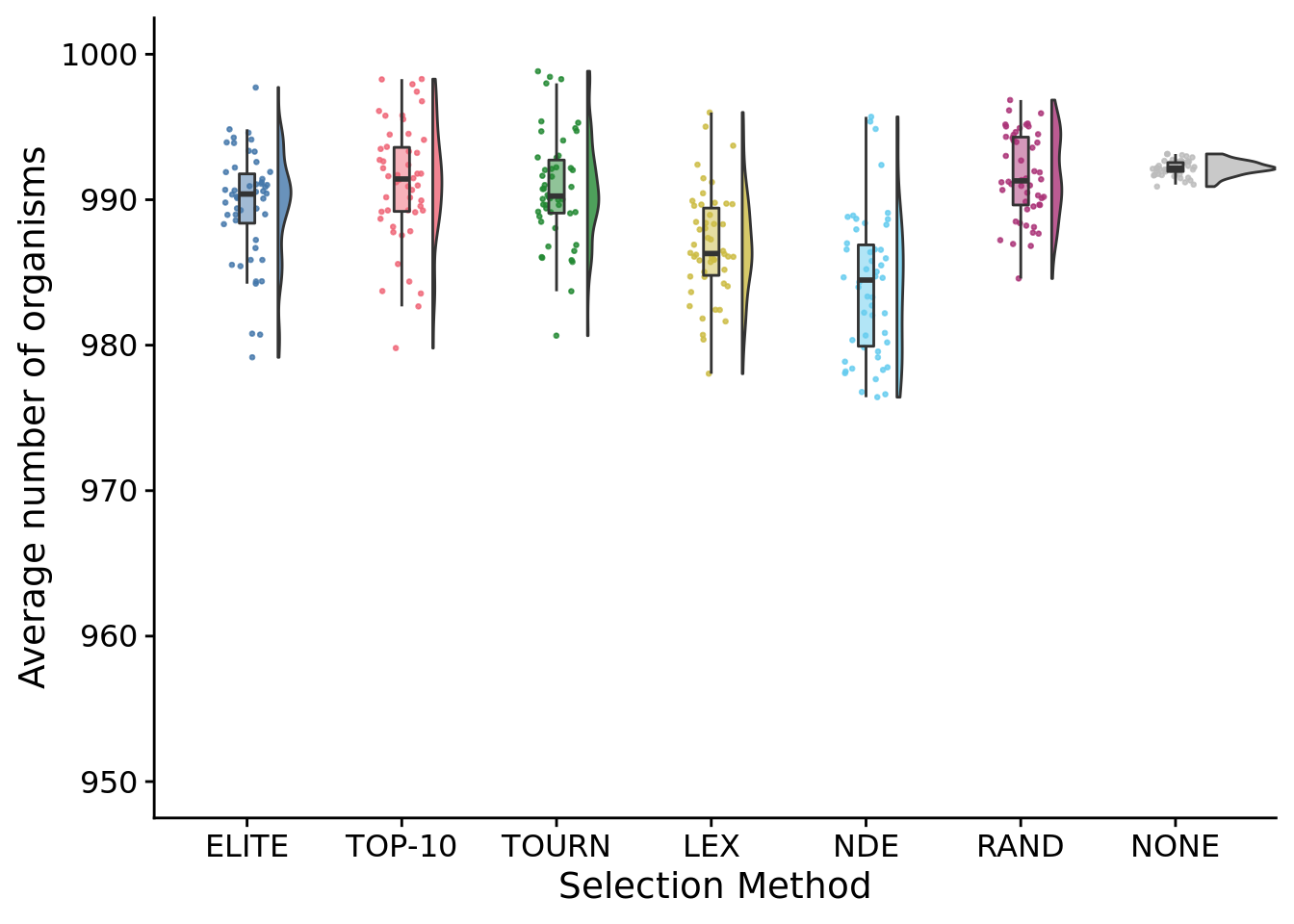
7.9 Average number of organisms in populations at end of maturation period
ggplot(
    exp_summary_data,
    aes(
      x=SELECTION_METHOD,
      y=avg_num_orgs,
      fill=SELECTION_METHOD
    )
  ) +
  geom_flat_violin(
    position = position_nudge(x = .2, y = 0),
    alpha = .8
  ) +
  geom_point(
    mapping=aes(color=SELECTION_METHOD),
    position = position_jitter(width = .15),
    size = .5,
    alpha = 0.8
  ) +
  geom_boxplot(
    width = .1,
    outlier.shape = NA,
    alpha = 0.5
  ) +
  scale_y_continuous(
    name="Average number of organisms",
    limits=c(950, 1000)
  ) +
  scale_x_discrete(
    name="Selection Method",
    breaks=selection_method_breaks,
    labels=selection_method_labels
  ) +
  scale_fill_fun(
  ) +
  scale_color_fun(
  ) +
  theme(
    legend.position="none"
  )
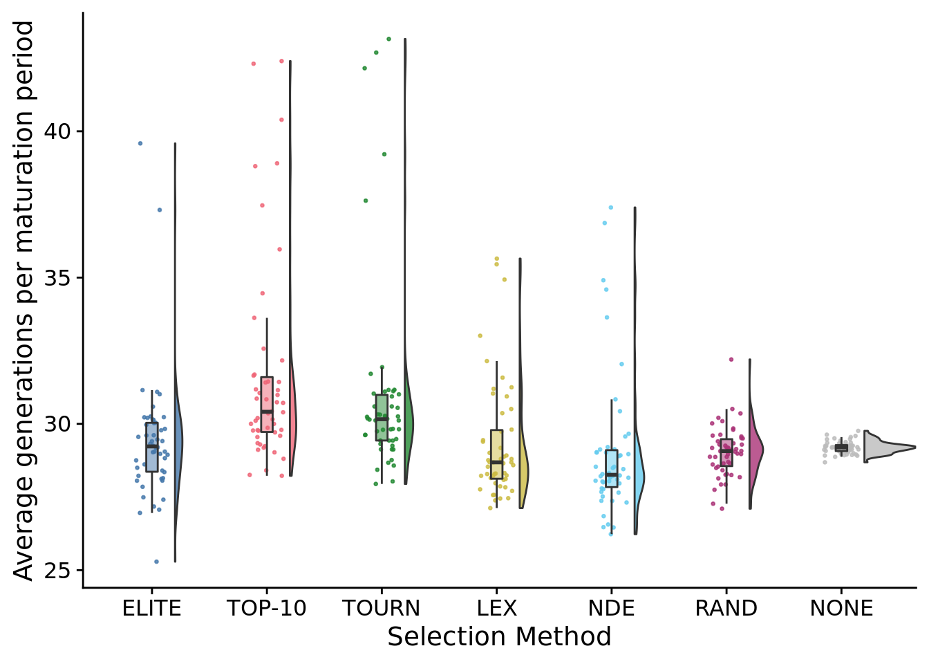
## Saving 7 x 5 in image7.10 Average generations per maturation period
ggplot(
    exp_summary_data,
    aes(
      x=SELECTION_METHOD,
      y=avg_gens,
      fill=SELECTION_METHOD
    )
  ) +
  geom_flat_violin(
    position = position_nudge(x = .2, y = 0),
    alpha = .8
  ) +
  geom_point(
    mapping=aes(color=SELECTION_METHOD),
    position = position_jitter(width = .15),
    size = .5,
    alpha = 0.8
  ) +
  geom_boxplot(
    width = .1,
    outlier.shape = NA,
    alpha = 0.5
  ) +
  scale_y_continuous(
    name="Average generations per maturation period"
  ) +
  scale_x_discrete(
    name="Selection Method",
    breaks=selection_method_breaks,
    labels=selection_method_labels
  ) +
  scale_fill_fun(
  ) +
  scale_color_fun(
  ) +
  theme(
    legend.position="none"
  )
## Saving 7 x 5 in imagemedian(exp_summary_data$total_gens_approx) # Used for determining how many generations to run EC for## [1] 57365.677.11 Representative task profiles
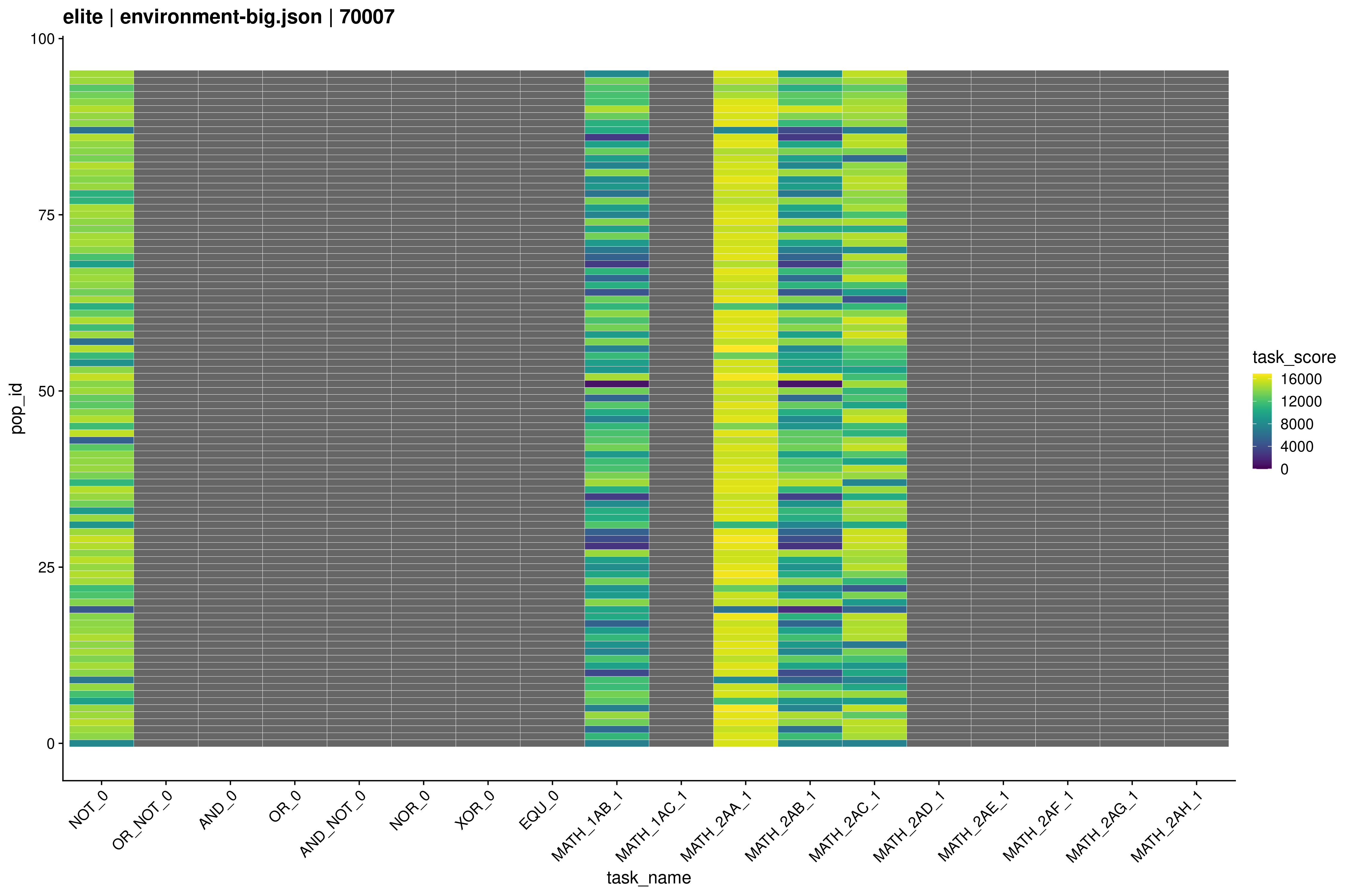
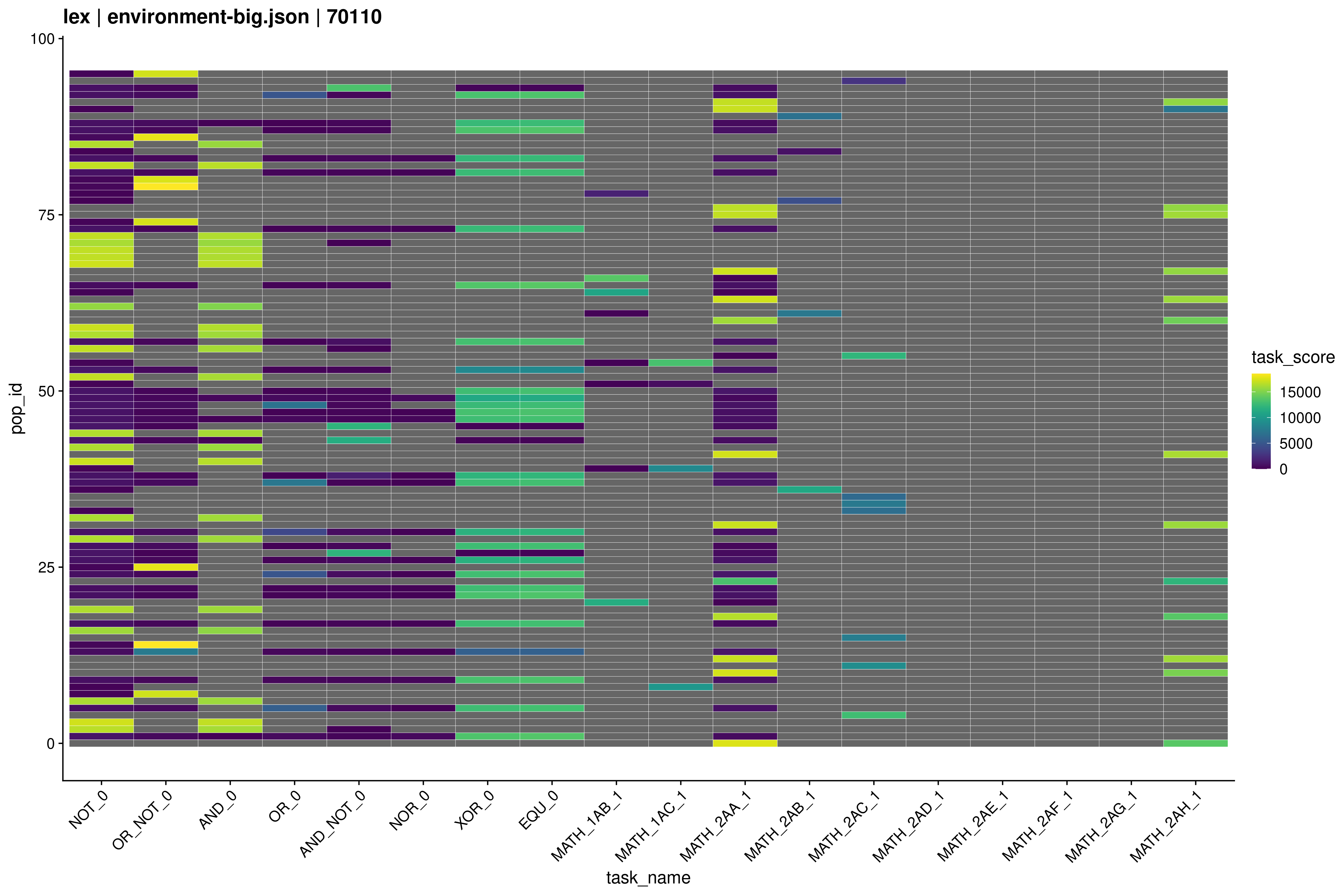
Visualized task profiles of two example metapopulations.
Elite selection
Lexicase selection
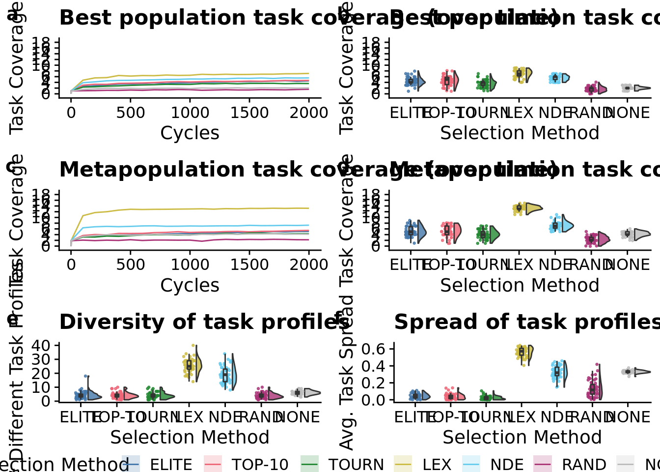
7.12 Manuscript figures
Without time series:
grid <- plot_grid(
  max_trait_cov_fig +
    theme(
      axis.title.x=element_blank(),
      axis.text=element_text(size=10),
      plot.title=element_text(size=12),
      axis.text.x = element_text(size = 9),
      axis.title.y = element_text(size = 10)
    ) +
    ggtitle("Best population task coverage"),
  total_trait_cov_fig +
    theme(
      axis.title.x=element_blank(),
      plot.title=element_text(size=12),
      axis.text=element_text(size=10),
      axis.text.x = element_text(size = 9),
      axis.title.y = element_text(size = 10)
    ) +
    ggtitle("Metapopulation task coverage"),
  num_pop_task_profiles_fig +
    theme(
      axis.text=element_text(size=10),
      plot.title=element_text(size=12),
      axis.text.x = element_text(size = 9),
      axis.title.y = element_text(size = 10)
    ) +
    ggtitle("Diversity of task profiles"),
  task_profile_spread_fig +
    theme(
      axis.text=element_text(size=10),
      plot.title=element_text(size=12),
      axis.text.x = element_text(size = 9),
      axis.title.y = element_text(size = 10)
    ) +
    ggtitle("Spread of task profiles"),
  nrow=2,
  ncol=2,
  labels="auto"
)
grid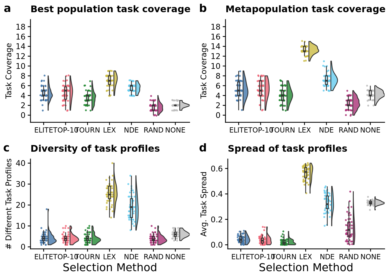
save_plot(
  filename=paste0(plot_directory, "2021-11-11-selection-figure.pdf"),
  plot=grid,
  base_height=5,
  base_asp=2.5,
  dpi=600
)
With time series:
legend <- cowplot::get_legend(
    max_trait_cov_ot_fig +
      guides(
        color=guide_legend(nrow=1),
        fill=guide_legend(nrow=1)
      ) +
      theme(
        legend.position = "bottom",
        legend.box="horizontal",
        legend.justification="center"
      )
  )
## Warning: Computation failed in `stat_summary()`:max_trait_cov_row <- plot_grid(
max_trait_cov_ot_fig +
ggtitle("Best population task coverage (over time)") +
theme(
legend.position="none"
# plot.title=element_text(size=12),
# axis.text=element_text(size=10),
# axis.text.x = element_text(size = 9),
# axis.title.y = element_text(size = 10)
),
max_trait_cov_fig +
ggtitle("Best population task coverage (final)"),
theme(
legend.position="none"
# plot.title=element_text(size=12),
# axis.text=element_text(size=10),
# axis.text.x = element_text(size = 9),
# axis.title.y = element_text(size = 10)
),
nrow=1,
ncol=2,
align="h",
labels=c("a", "b")
# rel_widths=c(3,2),
)## Warning: Computation failed in `stat_summary()`:## Warning in as_grob.default(plot): Cannot convert object of class themegg into a
## grob.## Warning: Graphs cannot be horizontally aligned unless the axis parameter is set.
## Placing graphs unaligned.# max_trait_cov_row
total_trait_cov_row <- plot_grid(
metapop_task_cov_ot_fig +
ggtitle("Metapopulation task coverage (over time)") +
theme(
legend.position="none"
# plot.title=element_text(size=12),
# axis.text=element_text(size=10),
# axis.text.x = element_text(size = 9),
# axis.title.y = element_text(size = 10)
),
total_trait_cov_fig +
ggtitle("Metapopulation task coverage (final)"),
theme(
legend.position="none"
# plot.title=element_text(size=12),
# axis.text=element_text(size=10),
# axis.text.x = element_text(size = 9),
# axis.title.y = element_text(size = 10)
),
nrow=1,
ncol=2,
align="h",
labels=c("c", "d")
# rel_widths=c(3,2),
)## Warning: Computation failed in `stat_summary()`:## Warning in as_grob.default(plot): Cannot convert object of class themegg into a
## grob.## Warning: Graphs cannot be horizontally aligned unless the axis parameter is set.
## Placing graphs unaligned.# total_trait_cov_row
diversity_row <- plot_grid(
num_pop_task_profiles_fig +
ggtitle("Diversity of task profiles") +
theme(
legend.position="none"
# plot.title=element_text(size=12),
# axis.text=element_text(size=10),
# axis.text.x = element_text(size = 9),
# axis.title.y = element_text(size = 10)
),
task_profile_spread_fig +
ggtitle("Spread of task profiles"),
theme(
legend.position="none"
# plot.title=element_text(size=12),
# axis.text=element_text(size=10),
# axis.text.x = element_text(size = 9),
# axis.title.y = element_text(size = 10)
),
nrow=1,
ncol=2,
align="h",
labels=c("e", "f")
# rel_widths=c(3,2),
)## Warning in as_grob.default(plot): Cannot convert object of class themegg into a
## grob.
## Warning in as_grob.default(plot): Graphs cannot be horizontally aligned unless
## the axis parameter is set. Placing graphs unaligned.# diversity_row
grid <- plot_grid(
max_trait_cov_row,
total_trait_cov_row,
diversity_row,
legend,
nrow=4,
ncol=1,
rel_heights=c(1, 1, 1, 0.1)
)
grid