Chapter 10 Varied genome lengths

10.1 Overview

In our main experiments, we limited genome length to 100 instructions. We ran a supplemental experiment to evaluate whether this limit substantially affected the directed evolution performance. Specifically, for each of elite and lexicase selection, we ran 30 replicates of digital directed evolution with the following genome length configurations: 50, 100 (default used in our main experiments), 150, and 200.

Note that these runs were performed with a maturation period of 300 updates and run for a total of 3,000 cycles (instead of 200 and 2,000, respectively).

experiment_slug <- "2021-11-08-longer-genomes"

working_directory <- paste0("experiments/",experiment_slug,"/analysis/")

10.2 Analysis dependencies

Load all required R libraries

library(tidyverse)
library(ggplot2)
library(cowplot)
library(RColorBrewer)
library(scales)
library(khroma)
source("https://gist.githubusercontent.com/benmarwick/2a1bb0133ff568cbe28d/raw/fb53bd97121f7f9ce947837ef1a4c65a73bffb3f/geom_flat_violin.R")

These analyses were knit with the following environment:

print(version)

##                _                           
## platform       x86_64-pc-linux-gnu         
## arch           x86_64                      
## os             linux-gnu                   
## system         x86_64, linux-gnu           
## status                                     
## major          4                           
## minor          2.1                         
## year           2022                        
## month          06                          
## day            23                          
## svn rev        82513                       
## language       R                           
## version.string R version 4.2.1 (2022-06-23)
## nickname       Funny-Looking Kid

10.3 Setup

Experiment summary data

exp_summary_data_loc <- paste0(working_directory,"data/experiment_summary.csv")
exp_summary_data <- read.csv(exp_summary_data_loc, na.strings="NONE")

exp_summary_data$SELECTION_METHOD <- factor(
  exp_summary_data$SELECTION_METHOD,
  levels=c(
    "elite",
    "tournament",
    "lexicase",
    "non-dominated-elite",
    "non-dominated-tournament",
    "random",
    "none"
  ),
  labels=c(
    "elite",
    "tourn",
    "lex",
    "nde",
    "ndt",
    "random",
    "none"
  )
)

exp_summary_data$AVIDAGP_ENV_FILE <- factor(
  exp_summary_data$AVIDAGP_ENV_FILE,
  levels=c(
    "environment-no-indiv.json",
    "environment-big.json"
  ),
  labels=c(
    "env-bb-0",
    "env-bb-1"
  )
)


exp_summary_data$NUM_POPS <- factor(
  exp_summary_data$NUM_POPS,
  levels=c(
    "24",
    "48",
    "96"
  )
)

exp_summary_data$UPDATES_PER_EPOCH <- as.factor(
  exp_summary_data$UPDATES_PER_EPOCH
)

exp_summary_data$TOURNAMENT_SEL_TOURN_SIZE <- as.factor(
  exp_summary_data$TOURNAMENT_SEL_TOURN_SIZE
)

exp_summary_data$POPULATION_SAMPLING_SIZE <- as.factor(
  exp_summary_data$POPULATION_SAMPLING_SIZE
)

exp_summary_data$genome_length <- factor(
  exp_summary_data$ANCESTOR_FILE,
  levels=c(
    "ancestor-50.gen",
    "ancestor-100.gen",
    "ancestor-150.gen",
    "ancestor-200.gen"
  ),
  labels=c(
    "50",
    "100",
    "150",
    "200"
  )
)

exp_summary_data$SAMPLE_SIZE <- exp_summary_data$POPULATION_SAMPLING_SIZE
exp_summary_data$ENV <- exp_summary_data$AVIDAGP_ENV_FILE
exp_summary_data$U_PER_E <- exp_summary_data$UPDATES_PER_EPOCH

Miscellaneous setup

# Configure our default graphing theme
theme_set(theme_cowplot())
# Create a directory to store plots
plot_directory <- paste0(working_directory, "plots/")
dir.create(plot_directory, showWarnings=FALSE)

selection_methods_smaller_set_colors <- c("#4477AA", "#CCBB44")

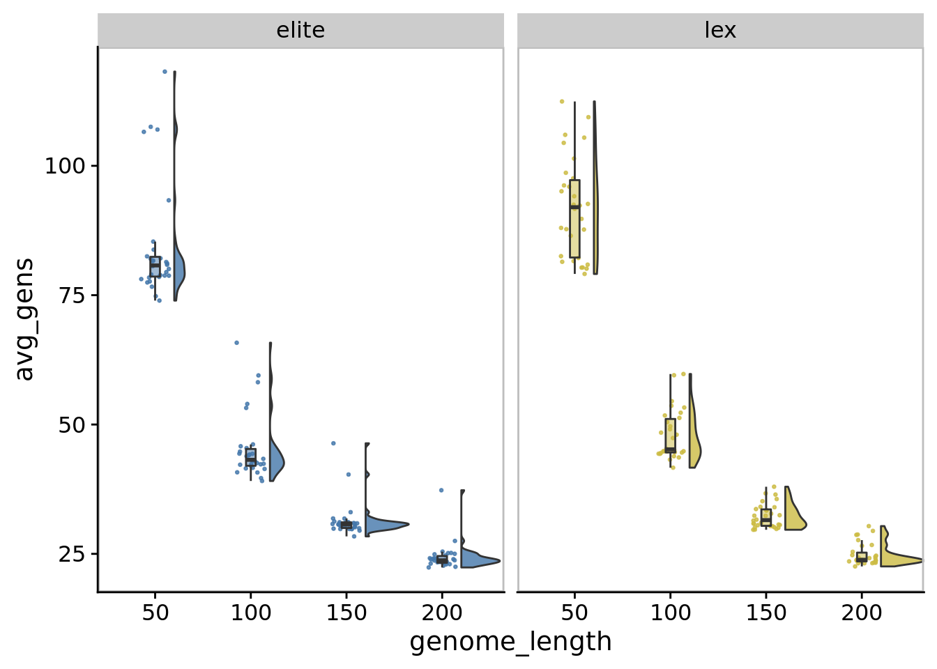
10.4 Average generations per maturation period

ggplot(
    exp_summary_data,
    aes(
      x=genome_length,
      y=avg_gens,
      fill=SELECTION_METHOD
    )
  ) +
  geom_flat_violin(
    position = position_nudge(x = .2, y = 0),
    alpha = .8
  ) +
  geom_point(
    mapping=aes(color=SELECTION_METHOD),
    position = position_jitter(width = .15),
    size = .5,
    alpha = 0.8
  ) +
  geom_boxplot(
    width = .1,
    outlier.shape = NA,
    alpha = 0.5
  ) +
  scale_fill_manual(
    values=selection_methods_smaller_set_colors
  ) +
  scale_color_manual(
    values=selection_methods_smaller_set_colors
  ) +
  facet_wrap(
    ~SELECTION_METHOD
  ) +
  theme(
    legend.position="none",
    panel.border=element_rect(colour="grey",size=1)
  )

ggsave(
  paste0(plot_directory, "avg_gens.pdf"),
  width=10,
  height=15
)

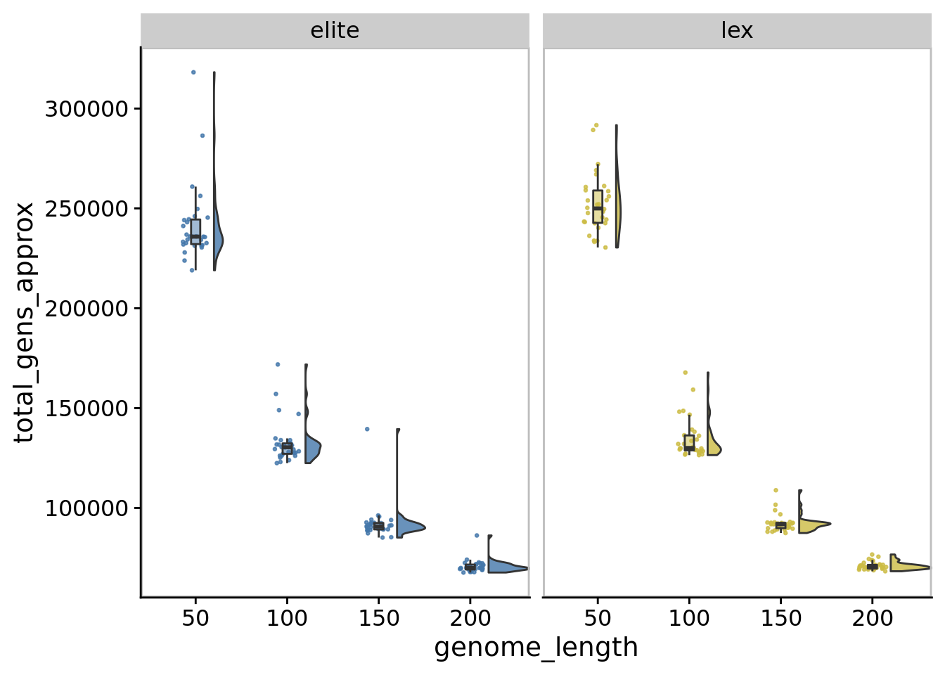
10.5 Total generations over experiment

ggplot(
    exp_summary_data,
    aes(
      x=genome_length,
      y=total_gens_approx,
      fill=SELECTION_METHOD
    )
  ) +
  geom_flat_violin(
    position = position_nudge(x = .2, y = 0),
    alpha = .8
  ) +
  geom_point(
    mapping=aes(color=SELECTION_METHOD),
    position = position_jitter(width = .15),
    size = .5,
    alpha = 0.8
  ) +
  geom_boxplot(
    width = .1,
    outlier.shape = NA,
    alpha = 0.5
  ) +
  scale_fill_manual(
    values=selection_methods_smaller_set_colors
  ) +
  scale_color_manual(
    values=selection_methods_smaller_set_colors
  ) +
  facet_wrap(
    ~SELECTION_METHOD
  ) +
  theme(
    legend.position="none",
    panel.border=element_rect(colour="grey",size=1)
  )

ggsave(
  paste0(plot_directory, "total_gens_approx.pdf"),
  width=10,
  height=15
)

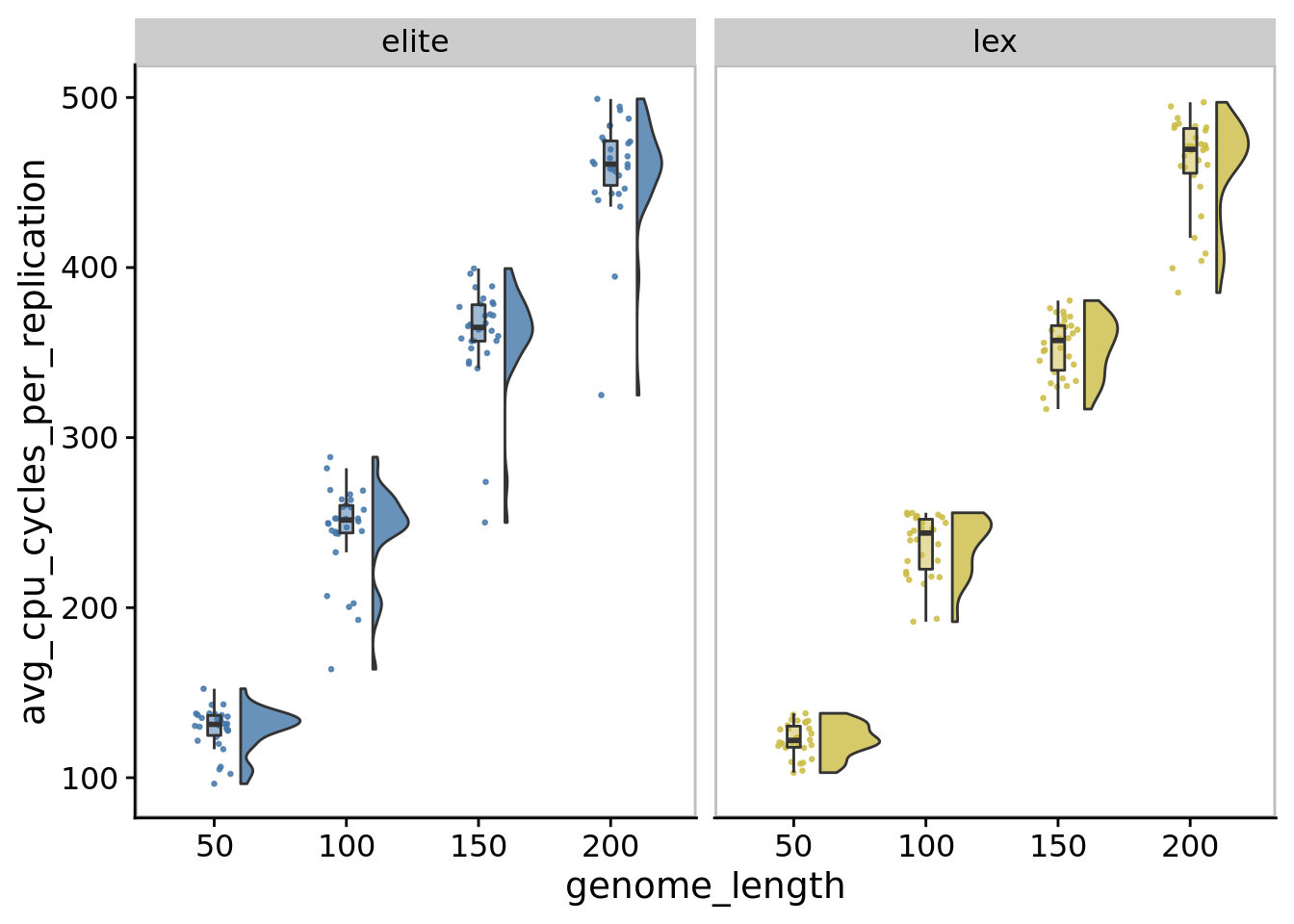
10.6 Performance

10.6.1 CPU cycles per replication

ggplot(
    exp_summary_data,
    aes(
      x=genome_length,
      y=avg_cpu_cycles_per_replication,
      fill=SELECTION_METHOD
    )
  ) +
  geom_flat_violin(
    position = position_nudge(x = .2, y = 0),
    alpha = .8
  ) +
  geom_point(
    mapping=aes(color=SELECTION_METHOD),
    position = position_jitter(height=0, width = .15),
    size = .5,
    alpha = 0.8
  ) +
  geom_boxplot(
    width = .1,
    outlier.shape = NA,
    alpha = 0.5
  ) +
  scale_fill_manual(
    values=selection_methods_smaller_set_colors
  ) +
  scale_color_manual(
    values=selection_methods_smaller_set_colors
  ) +
  facet_wrap(
    ~SELECTION_METHOD
  ) +
  theme(
    legend.position="none",
    panel.border=element_rect(colour="grey",size=1)
  )

ggsave(
  paste0(plot_directory, "avg_cpu_cycles_per_replication.pdf")
)

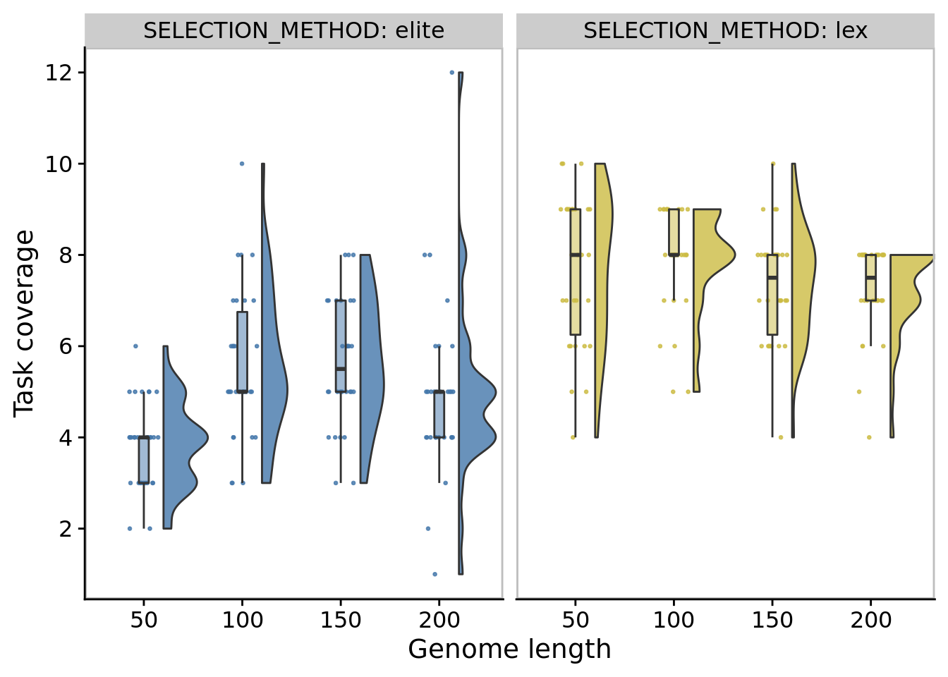
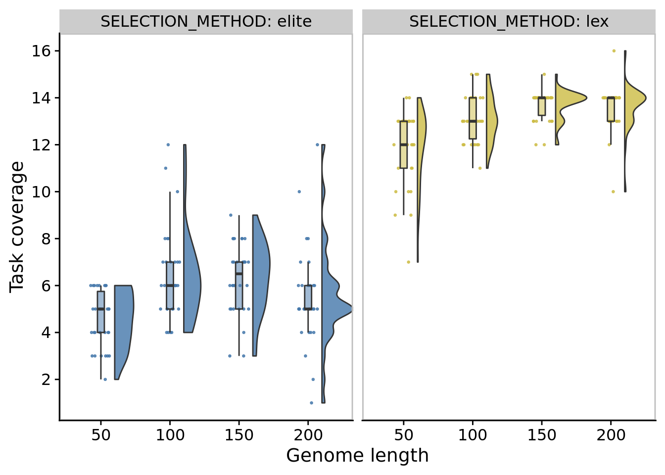
## Saving 7 x 5 in image

10.6.2 Best single-population task coverage

ggplot(
    exp_summary_data,
    aes(
      x=genome_length,
      y=max_trait_coverage,
      fill=SELECTION_METHOD
    )
  ) +
  geom_flat_violin(
    position = position_nudge(x = .2, y = 0),
    alpha = .8
  ) +
  geom_point(
    mapping=aes(color=SELECTION_METHOD),
    position = position_jitter(height=0, width = .15),
    size = .5,
    alpha = 0.8
  ) +
  geom_boxplot(
    width = .1,
    outlier.shape = NA,
    alpha = 0.5
  ) +
  scale_x_discrete(
    name="Genome length"
  ) +
  scale_y_continuous(
    name="Task coverage",
    breaks=seq(0,18,2)
  ) +
  scale_fill_manual(
    values=selection_methods_smaller_set_colors
  ) +
  scale_color_manual(
    values=selection_methods_smaller_set_colors
  ) +
  facet_wrap(
    ~SELECTION_METHOD,
    nrow=1,
    labeller=label_both
  ) +
  theme(
    legend.position="none",
    panel.border=element_rect(colour="grey",size=1)
  )

ggsave(
  paste0(plot_directory, "2021-11-08-best-pop-task-cov.pdf"),
  width=8,
  height=4
)

10.6.3 Metapopulation task coverage

ggplot(
    exp_summary_data,
    aes(
      x=genome_length,
      y=total_trait_coverage,
      fill=SELECTION_METHOD
    )
  ) +
  geom_flat_violin(
    position = position_nudge(x = .2, y = 0),
    alpha = .8
  ) +
  geom_point(
    mapping=aes(color=SELECTION_METHOD),
    position = position_jitter(height=0, width = .15),
    size = .5,
    alpha = 0.8
  ) +
  geom_boxplot(
    width = .1,
    outlier.shape = NA,
    alpha = 0.5
  ) +
  scale_x_discrete(
    name="Genome length"
  ) +
  scale_y_continuous(
    name="Task coverage",
    breaks=seq(0,18,2)
  ) +
  scale_fill_manual(
    values=selection_methods_smaller_set_colors
  ) +
  scale_color_manual(
    values=selection_methods_smaller_set_colors
  ) +
  facet_wrap(
    ~SELECTION_METHOD,
    nrow=1,
    labeller=label_both
  ) +
  theme(
    legend.position="none",
    panel.border=element_rect(colour="grey",size=1)
  )

ggsave(
  paste0(plot_directory, "2021-11-08-metapop-task-cov.pdf"),
  width=8,
  height=4
)

10.7 Population-level task profile diversity

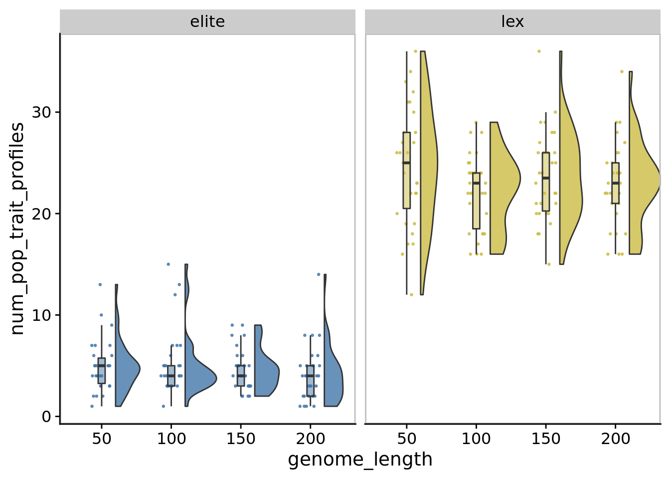
10.7.1 Task profile richness

ggplot(
    exp_summary_data,
    aes(
      x=genome_length,
      y=num_pop_trait_profiles,
      fill=SELECTION_METHOD
    )
  ) +
  geom_flat_violin(
    position = position_nudge(x = .2, y = 0),
    alpha = .8
  ) +
  geom_point(
    mapping=aes(color=SELECTION_METHOD),
    position = position_jitter(height=0, width = .15),
    size = .5,
    alpha = 0.8
  ) +
  geom_boxplot(
    width = .1,
    outlier.shape = NA,
    alpha = 0.5
  ) +
  scale_fill_manual(
    values=selection_methods_smaller_set_colors
  ) +
  scale_color_manual(
    values=selection_methods_smaller_set_colors
  ) +
  facet_wrap(
    ~SELECTION_METHOD
  ) +
  theme(
    legend.position="none",
    panel.border=element_rect(colour="grey",size=1)
  )

ggsave(
  paste0(plot_directory, "num_pop_trait_profiles.pdf")
)

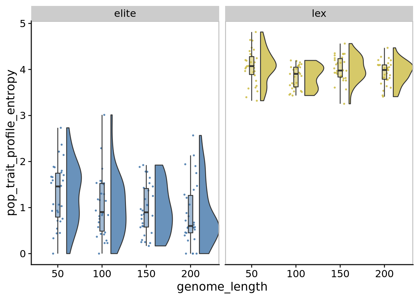
## Saving 7 x 5 in image

10.7.2 Task profile entropy

ggplot(
    exp_summary_data,
    aes(
      x=genome_length,
      y=pop_trait_profile_entropy,
      fill=SELECTION_METHOD
    )
  ) +
  geom_flat_violin(
    position = position_nudge(x = .2, y = 0),
    alpha = .8
  ) +
  geom_point(
    mapping=aes(color=SELECTION_METHOD),
    position = position_jitter(height=0, width = .15),
    size = .5,
    alpha = 0.8
  ) +
  geom_boxplot(
    width = .1,
    outlier.shape = NA,
    alpha = 0.5
  ) +
  scale_fill_manual(
    values=selection_methods_smaller_set_colors
  ) +
  scale_color_manual(
    values=selection_methods_smaller_set_colors
  ) +
  facet_wrap(
    ~SELECTION_METHOD
  ) +
  theme(
    legend.position="none",
    panel.border=element_rect(colour="grey",size=1)
  )

ggsave(
  paste0(plot_directory, "pop_trait_profile_entropy.pdf")
)

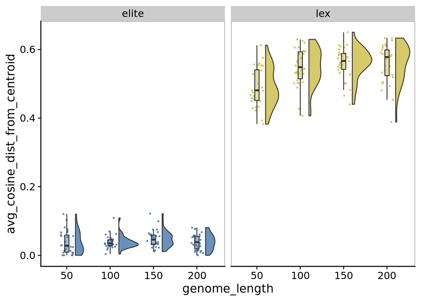
## Saving 7 x 5 in image

10.7.3 Spread (avg cosine distance)

ggplot(
    exp_summary_data,
    aes(
      x=genome_length,
      y=avg_cosine_dist_from_centroid,
      fill=SELECTION_METHOD
    )
  ) +
  geom_flat_violin(
    position = position_nudge(x = .2, y = 0),
    alpha = .8
  ) +
  geom_point(
    mapping=aes(color=SELECTION_METHOD),
    position = position_jitter(height=0, width = .15),
    size = .5,
    alpha = 0.8
  ) +
  geom_boxplot(
    width = .1,
    outlier.shape = NA,
    alpha = 0.5
  ) +
  scale_fill_manual(
    values=selection_methods_smaller_set_colors
  ) +
  scale_color_manual(
    values=selection_methods_smaller_set_colors
  ) +
  facet_wrap(
    ~SELECTION_METHOD
  ) +
  theme(
    legend.position="none",
    panel.border=element_rect(colour="grey",size=1)
  )

ggsave(
  paste0(plot_directory, "avg_cosine_dist_from_centroid.pdf")
)

## Saving 7 x 5 in image

10.8 Selection

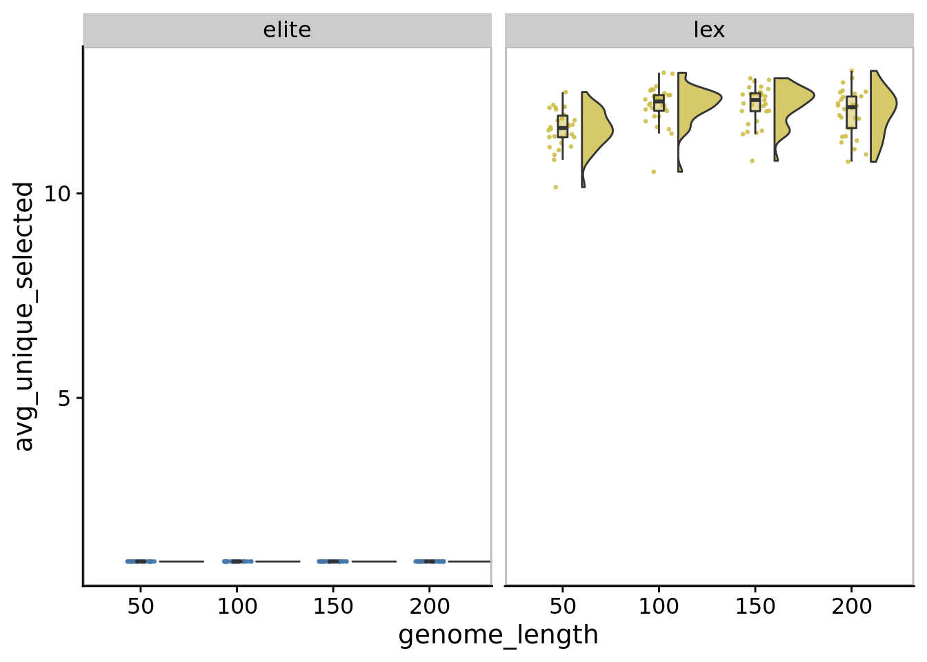
10.8.1 Average number of unique populations selected

ggplot(
    exp_summary_data,
    aes(
      x=genome_length,
      y=avg_unique_selected,
      fill=SELECTION_METHOD
    )
  ) +
  geom_flat_violin(
    position = position_nudge(x = .2, y = 0),
    alpha = .8
  ) +
  geom_point(
    mapping=aes(color=SELECTION_METHOD),
    position = position_jitter(height=0, width = .15),
    size = .5,
    alpha = 0.8
  ) +
  geom_boxplot(
    width = .1,
    outlier.shape = NA,
    alpha = 0.5
  ) +
  scale_fill_manual(
    values=selection_methods_smaller_set_colors
  ) +
  scale_color_manual(
    values=selection_methods_smaller_set_colors
  ) +
  facet_wrap(
    ~SELECTION_METHOD
  ) +
  theme(
    legend.position="none",
    panel.border=element_rect(colour="grey",size=1)
  )

ggsave(
  paste0(plot_directory, "avg_unique_selected.pdf")
)

## Saving 7 x 5 in image

10.8.2 Average entropy of selection ids

ggplot(
    exp_summary_data,
    aes(
      x=genome_length,
      y=avg_entropy_selected,
      fill=SELECTION_METHOD
    )
  ) +
  geom_flat_violin(
    position = position_nudge(x = .2, y = 0),
    alpha = .8
  ) +
  geom_point(
    mapping=aes(color=SELECTION_METHOD),
    position = position_jitter(height=0, width = .15),
    size = .5,
    alpha = 0.8
  ) +
  geom_boxplot(
    width = .1,
    outlier.shape = NA,
    alpha = 0.5
  ) +
  scale_fill_manual(
    values=selection_methods_smaller_set_colors
  ) +
  scale_color_manual(
    values=selection_methods_smaller_set_colors
  ) +
  facet_wrap(
    ~SELECTION_METHOD
  ) +
  theme(
    legend.position="none",
    panel.border=element_rect(colour="grey",size=1)
  )

ggsave(
  paste0(plot_directory, "avg_entropy_selected.pdf")
)

## Saving 7 x 5 in image

10.9 Discussion

The task performance data show that our chosen genome length of 100 is a reasonable choice, as there are not substantial performance improvements with longer genome lengths.