Chapter 11 Population propagule sample size

In this preliminary experiment, we looked at the effect of varying the size of propagules used when creating “offspring” populations from “parent” populations.

We conducted these exploratory experiments well before the final set of experiments presented in our manuscript, so their setups are not the same:

• We only compared elite, lexicase, non-dominated elite, and a no selection control.
• The environment is simpler with 8 population-level functions instead of 18.
• The maximum population size is 900 instead of 1,000.
• The maturation period is longer (300 updates versus 200)
• We ran the experiment for fewer cycles (500 instead of 2,000).

Overall, we found that the effect of propagule size varied by selection scheme. For elite selection and the no-selection control, sample size had little effect. For lexicase and non-dominated elite selection, the smallest propagule size (1% of the maximum population size) resulted in significantly better outcomes than using larger propagule sizes (e.g., 100% of the maximum population size).

Because these data were collected during early experiments, we tracked fewer population/metapopulation statistics. Future work should further investigate the effects of propagule size, especially in the context of more complex environments that support more complex organism-organism interaction.

11.1 Overview

experiment_slug <- "2021-09-30-sample-size"

working_directory <- paste0("experiments/",experiment_slug,"/analysis/")

11.2 Analysis dependencies

Load all required R libraries

library(tidyverse)
library(ggplot2)
library(cowplot)
library(RColorBrewer)
library(scales)
library(khroma)
source("https://gist.githubusercontent.com/benmarwick/2a1bb0133ff568cbe28d/raw/fb53bd97121f7f9ce947837ef1a4c65a73bffb3f/geom_flat_violin.R")

These analyses were knit with the following environment:

print(version)

##                _                           
## platform       x86_64-pc-linux-gnu         
## arch           x86_64                      
## os             linux-gnu                   
## system         x86_64, linux-gnu           
## status                                     
## major          4                           
## minor          2.1                         
## year           2022                        
## month          06                          
## day            23                          
## svn rev        82513                       
## language       R                           
## version.string R version 4.2.1 (2022-06-23)
## nickname       Funny-Looking Kid

11.3 Setup

Experiment summary data

exp_summary_data_loc <- paste0(working_directory,"data/experiment_summary.csv")
exp_summary_data <- read.csv(exp_summary_data_loc, na.strings="NONE")

# Mark factors
exp_summary_data$SELECTION_METHOD <- factor(
  exp_summary_data$SELECTION_METHOD,
  levels=c(
    "elite",
    "tournament",
    "lexicase",
    "non-dominated-elite",
    "non-dominated-tournament",
    "random",
    "none"
  ),
  labels=c(
    "elite",
    "tournament",
    "lex",
    "nde",
    "ndt",
    "random",
    "none"
  )
)

exp_summary_data$NUM_POPS <- factor(
  exp_summary_data$NUM_POPS,
  levels=c(
    "24",
    "48",
    "96"
  )
)

exp_summary_data$UPDATES_PER_EPOCH <- as.factor(
  exp_summary_data$UPDATES_PER_EPOCH
)

exp_summary_data$POPULATION_SAMPLING_SIZE <- as.factor(
  exp_summary_data$POPULATION_SAMPLING_SIZE
)

exp_summary_data$SAMPLE_SIZE <- exp_summary_data$POPULATION_SAMPLING_SIZE

exp_summary_data <- filter(exp_summary_data, UPDATES_PER_EPOCH=="300")

Miscellaneous setup

# Configure our default graphing theme
theme_set(theme_cowplot())
# Create a directory to store plots
plot_directory <- paste0(working_directory, "plots/")
dir.create(plot_directory, showWarnings=FALSE)

selection_methods_smaller_set_colors <- c("#4477AA", "#CCBB44", "#66CCEE", "#BBBBBB")

sel.labs <- c(
  "elite",
  "tournament",
  "lex",
  "nde",
  "ndt",
  "random",
  "none"
)
names(sel.labs) <- c(
  "elite",
  "tournament",
  "lex",
  "nde",
  "ndt",
  "random",
  "none"
)
upe.labs <- c(
  "updates per cycle=100",
  "updates per cycle=300"
)
names(upe.labs) <- c(
  "100",
  "300"
)

11.4 Average number of organisms

Average number of organisms per world at the end of a run.

ggplot(
    exp_summary_data,
    aes(
      x=POPULATION_SAMPLING_SIZE,
      y=avg_num_orgs,
      fill=SELECTION_METHOD
    )
  ) +
  geom_flat_violin(
    position = position_nudge(x = .2, y = 0),
    alpha = .8
  ) +
  geom_point(
    mapping=aes(color=SELECTION_METHOD),
    position = position_jitter(width = .15),
    size = .5,
    alpha = 0.8
  ) +
  geom_boxplot(
    width = .1,
    outlier.shape = NA,
    alpha = 0.5
  ) +
  scale_fill_manual(
    values=selection_methods_smaller_set_colors
  ) +
  scale_color_manual(
    values=selection_methods_smaller_set_colors
  ) +
  facet_grid(
    UPDATES_PER_EPOCH~SELECTION_METHOD,
    labeller = labeller(UPDATES_PER_EPOCH=upe.labs, SELECTION_METHOD=sel.labs)
  ) +
  theme(
    legend.position="none",
    axis.text.x=element_text(angle=45,hjust=1)
  )

ggsave(
  paste0(plot_directory, "avg_num_orgs.pdf")
)

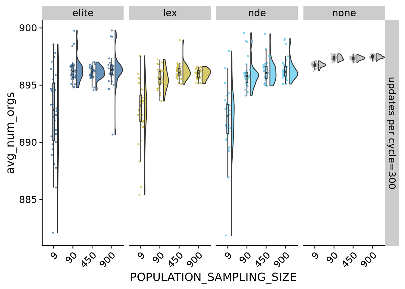
## Saving 7 x 5 in image

In general, the smaller propagule sizes are less likely to reach 900 organisms during the maturation period. However, all final population sizes are within 25 organisms of each, so no substantial differences here.

11.5 Average generations per maturation period

ggplot(
  exp_summary_data,
    aes(
      x=POPULATION_SAMPLING_SIZE,
      y=avg_gens,
      fill=SELECTION_METHOD
    )
  ) +
  geom_flat_violin(
    position = position_nudge(x = .2, y = 0),
    alpha = .8
  ) +
  geom_point(
    mapping=aes(color=SELECTION_METHOD),
    position = position_jitter(width = .15),
    size = .5,
    alpha = 0.8
  ) +
  geom_boxplot(
    width = .1,
    outlier.shape = NA,
    alpha = 0.5
  ) +
  scale_fill_manual(
    values=selection_methods_smaller_set_colors
  ) +
  scale_color_manual(
    values=selection_methods_smaller_set_colors
  ) +
  facet_grid(
    UPDATES_PER_EPOCH~SELECTION_METHOD,
    labeller = labeller(UPDATES_PER_EPOCH=upe.labs, SELECTION_METHOD=sel.labs)
  ) +
  theme(
    legend.position="none",
    axis.text.x=element_text(angle=45,hjust=1)
  )

ggsave(
  paste0(plot_directory, "avg_gens.pdf"),
  width=10,
  height=15
)

11.6 Performance

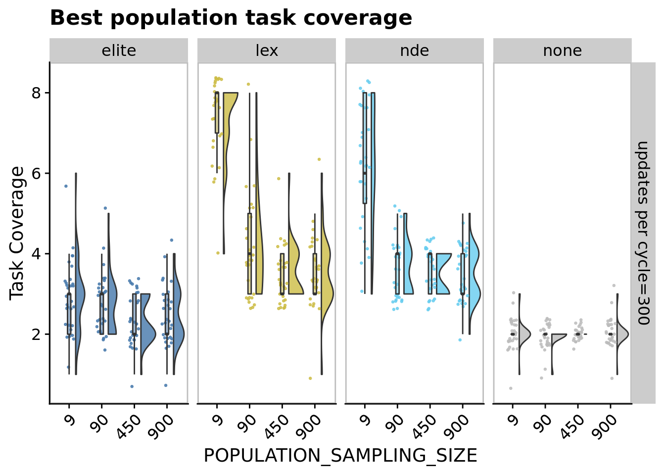
11.6.1 Best population task coverage

ggplot(
  exp_summary_data,
    aes(
      x=POPULATION_SAMPLING_SIZE,
      y=max_trait_coverage,
      fill=SELECTION_METHOD
    )
  ) +
  geom_flat_violin(
    position = position_nudge(x = .2, y = 0),
    alpha = .8
  ) +
  geom_point(
    mapping=aes(color=SELECTION_METHOD),
    position = position_jitter(width = .15),
    size = .5,
    alpha = 0.8
  ) +
  geom_boxplot(
    width = .1,
    outlier.shape = NA,
    alpha = 0.5
  ) +
  scale_y_continuous(
    name="Task Coverage"
  ) +
  scale_fill_manual(
    values=selection_methods_smaller_set_colors
  ) +
  scale_color_manual(
    values=selection_methods_smaller_set_colors
  ) +
  facet_grid(
    UPDATES_PER_EPOCH~SELECTION_METHOD,
    labeller = labeller(UPDATES_PER_EPOCH=upe.labs, SELECTION_METHOD=sel.labs)
  ) +
  ggtitle("Best population task coverage") +
  theme(
    legend.position="none",
    axis.text.x=element_text(angle=45,hjust=1),
    panel.border=element_rect(colour="grey",size=1)
  )

ggsave(
  paste0(plot_directory, "max_trait_coverage.png"),
  width=10,
  height=6
)

comp_data <- filter(
  exp_summary_data,
  SELECTION_METHOD=="lex"
)
kruskal.test(
  formula=max_trait_coverage~POPULATION_SAMPLING_SIZE,
  data=comp_data
)

## 
##  Kruskal-Wallis rank sum test
## 
## data:  max_trait_coverage by POPULATION_SAMPLING_SIZE
## Kruskal-Wallis chi-squared = 69.574, df = 3, p-value = 5.266e-15

pairwise.wilcox.test(
  x=comp_data$max_trait_coverage,
  g=comp_data$POPULATION_SAMPLING_SIZE,
  p.adjust.method="bonferroni",
  exact=FALSE
)

## 
##  Pairwise comparisons using Wilcoxon rank sum test with continuity correction 
## 
## data:  comp_data$max_trait_coverage and comp_data$POPULATION_SAMPLING_SIZE 
## 
##     9       90    450  
## 90  5.8e-09 -     -    
## 450 1.1e-10 0.091 -    
## 900 1.6e-10 0.241 1.000
## 
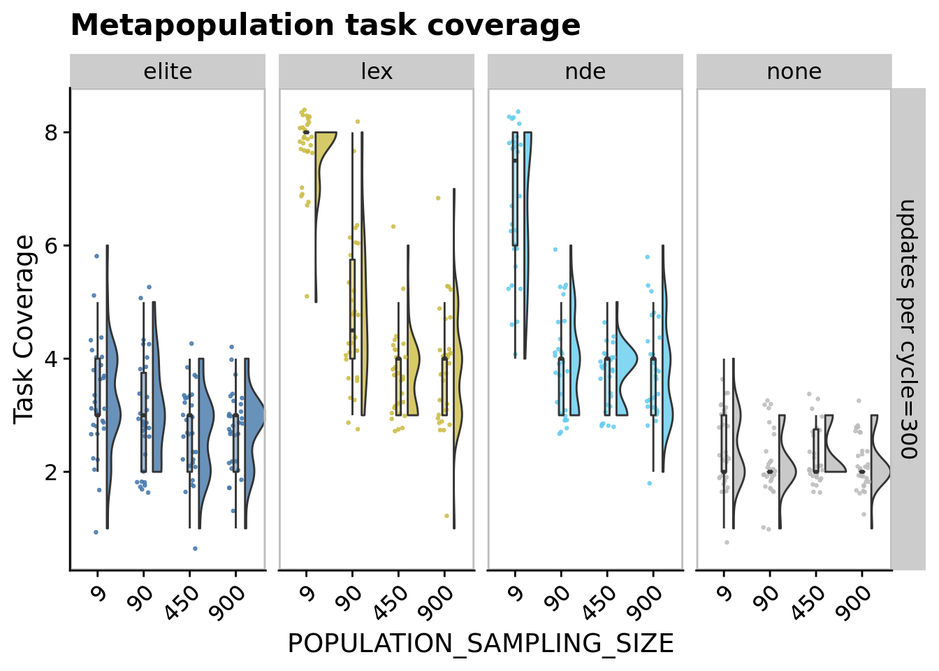
## P value adjustment method: bonferroni

11.6.2 Metapopulation task coverage

ggplot(
  exp_summary_data,
    aes(
      x=POPULATION_SAMPLING_SIZE,
      y=total_trait_coverage,
      fill=SELECTION_METHOD
    )
  ) +
  geom_flat_violin(
    position = position_nudge(x = .2, y = 0),
    alpha = .8
  ) +
  geom_point(
    mapping=aes(color=SELECTION_METHOD),
    position = position_jitter(width = .15),
    size = .5,
    alpha = 0.8
  ) +
  geom_boxplot(
    width = .1,
    outlier.shape = NA,
    alpha = 0.5
  ) +
  scale_y_continuous(
    name="Task Coverage"
  ) +
  scale_fill_manual(
    values=selection_methods_smaller_set_colors
  ) +
  scale_color_manual(
    values=selection_methods_smaller_set_colors
  ) +
  facet_grid(
    UPDATES_PER_EPOCH~SELECTION_METHOD,
    labeller = labeller(UPDATES_PER_EPOCH=upe.labs, SELECTION_METHOD=sel.labs)
  ) +
  ggtitle("Metapopulation task coverage") +
  theme(
    legend.position="none",
    axis.text.x=element_text(angle=45,hjust=1),
    panel.border=element_rect(colour="grey",size=1)
  )

ggsave(
  paste0(plot_directory, "total_trait_coverage.png"),
  width=10,
  height=6
)

comp_data <- filter(
  exp_summary_data,
  SELECTION_METHOD=="lex"
)
kruskal.test(
  formula=total_trait_coverage~POPULATION_SAMPLING_SIZE,
  data=comp_data
)

## 
##  Kruskal-Wallis rank sum test
## 
## data:  total_trait_coverage by POPULATION_SAMPLING_SIZE
## Kruskal-Wallis chi-squared = 74.497, df = 3, p-value = 4.644e-16

pairwise.wilcox.test(
  x=comp_data$total_trait_coverage,
  g=comp_data$POPULATION_SAMPLING_SIZE,
  p.adjust.method="bonferroni",
  exact=FALSE
)

## 
##  Pairwise comparisons using Wilcoxon rank sum test with continuity correction 
## 
## data:  comp_data$total_trait_coverage and comp_data$POPULATION_SAMPLING_SIZE 
## 
##     9       90     450   
## 90  2.2e-09 -      -     
## 450 2.3e-11 0.0012 -     
## 900 5.3e-11 0.0279 1.0000
## 
## P value adjustment method: bonferroni