Chapter 9 Varying population maturation period

9.1 Overview

How robust are our digital directed evolution results at different maturation periods? Adjusting the length of population maturation periods shifts the balance of individual-level and population-level selection pressure. Shorter maturation periods have shorter stints where organisms compete within a population between population-level selection events; whereas, longer maturation periods have longer stints where organisms are competing for space within a population before a population-level selection event occurs.

Naively, we might maximize selection pressure on population-level functions by minimizing maturation periods; however, maturation periods of organism-level evolution are important for accumulating genetic variation in a population. We could maximize genetic divergence among populations in a metapopulation by using long maturation periods; however, if population-level selection events are too infrequent, there may not be sufficient selection pressure to maintain population-level functions if they are not also sufficiently beneficial at the individual-level. We expect there to be an ideal maturation period length that will vary depending on the particular organisms and functions being evolved.

We ran a supplemental experiment to evaluate the robustness of our results at a range of maturation period lengths. For each of elite selection, lexicase selection, non-dominated elite selection, and no selection (control), we ran 50 replicates of digital directed evolution with the following maturation period lengths (given in updates): 20, 50, 100, 200 (the default used in our main experiments), 500, and 1,000. For each condition, we held the total number of updates constant (400,000 total updates); that is, we ran fewer overall cycles of directed evolution at larger maturation periods (e.g., 400 cycles for 1,000 update maturation periods), and a greater number of cycles at smaller maturation periods (e.g., 20,000 cycles for 20 update maturation periods). We used a more limited set of selection schemes for this supplemental experiment due to constraints on computing resources.

experiment_slug <- "2021-11-12-time"

working_directory <- paste0("experiments/",experiment_slug,"/analysis/")

9.2 Analysis dependencies

Load all required R libraries

library(tidyverse)
library(ggplot2)
library(cowplot)
library(RColorBrewer)
library(scales)

## 
## Attaching package: 'scales'

## The following object is masked from 'package:purrr':
## 
##     discard

## The following object is masked from 'package:readr':
## 
##     col_factor

library(khroma)
source("https://gist.githubusercontent.com/benmarwick/2a1bb0133ff568cbe28d/raw/fb53bd97121f7f9ce947837ef1a4c65a73bffb3f/geom_flat_violin.R")

These analyses were knit with the following environment:

print(version)

##                _                           
## platform       x86_64-pc-linux-gnu         
## arch           x86_64                      
## os             linux-gnu                   
## system         x86_64, linux-gnu           
## status                                     
## major          4                           
## minor          2.1                         
## year           2022                        
## month          06                          
## day            23                          
## svn rev        82513                       
## language       R                           
## version.string R version 4.2.1 (2022-06-23)
## nickname       Funny-Looking Kid

9.3 Setup

Experiment summary data

exp_summary_data_loc <- paste0(working_directory,"data/experiment_summary.csv")
exp_summary_data <- read.csv(exp_summary_data_loc, na.strings="NONE")

exp_summary_data$SELECTION_METHOD <- factor(
  exp_summary_data$SELECTION_METHOD,
  levels=c(
    "elite",
    "tournament",
    "lexicase",
    "non-dominated-elite",
    "non-dominated-tournament",
    "random",
    "none"
  ),
  labels=c(
    "elite",
    "tourn",
    "lex",
    "nde",
    "ndt",
    "random",
    "none"
  )
)

exp_summary_data$UPDATES_PER_EPOCH <- as.factor(
  exp_summary_data$UPDATES_PER_EPOCH
)

exp_summary_data$TOURNAMENT_SEL_TOURN_SIZE <- as.factor(
  exp_summary_data$TOURNAMENT_SEL_TOURN_SIZE
)

exp_summary_data$U_PER_E <- exp_summary_data$UPDATES_PER_EPOCH

Miscellaneous setup

# Configure our default graphing theme
theme_set(theme_cowplot())
# Palette
scale_fill_fun <- scale_fill_bright
scale_color_fun <- scale_color_bright
# Create a directory to store plots
plot_directory <- paste0(working_directory, "plots/")
dir.create(plot_directory, showWarnings=FALSE)

selection_method_breaks <- c("elite", "tourn", "lex", "nde", "random", "none")
selection_method_labels <- c("ELITE", "TOURN", "LEX", "NDE", "RAND", "NONE")

exp_summary_data$SELECTION_METHOD_LABEL <- factor(
  exp_summary_data$SELECTION_METHOD,
  levels=c(
    "elite",
    "tourn",
    "lex",
    "nde",
    "ndt",
    "random",
    "none"
  ),
  labels=c(
    "Elite Selection",
    "Tournament Selection",
    "Lexicase Selection",
    "Non-dominated Elite Selection",
    "Non-dominated Tournament Selection",
    "Random Selection",
    "No Selection"
  )
)
# 1, 4, 5, 7
selection_methods_smaller_set_colors <- c("#4477AA", "#CCBB44", "#66CCEE", "#BBBBBB")
# c("#66C2A5", "#E78AC3", "#A6D854", "#E5C494")
# c("#66C2A5", "#8DA0CB", "#E78AC3", "#FFD92F")

9.4 Average number of organisms

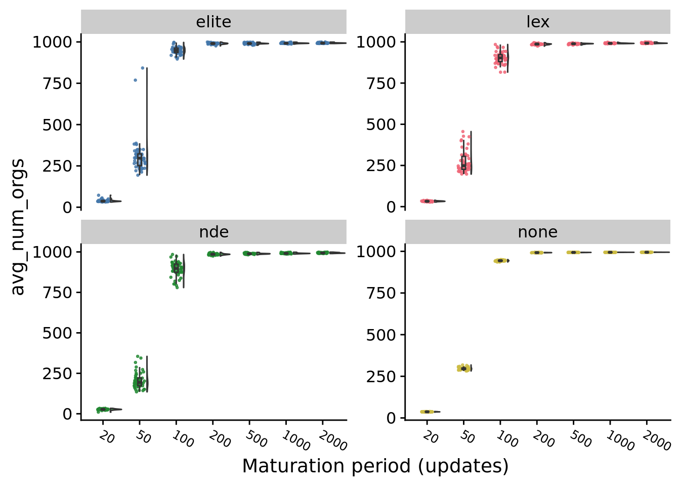
Average number of organisms per world at the end of a run.

ggplot(
    exp_summary_data,
    aes(
      x=U_PER_E,
      y=avg_num_orgs,
      fill=SELECTION_METHOD
    )
  ) +
  geom_flat_violin(
    position = position_nudge(x = .2, y = 0),
    alpha = .8
  ) +
  geom_point(
    mapping=aes(color=SELECTION_METHOD),
    position = position_jitter(width = .15),
    size = .5,
    alpha = 0.8
  ) +
  geom_boxplot(
    width = .1,
    outlier.shape = NA,
    alpha = 0.5
  ) +
  scale_x_discrete(
    name="Maturation period (updates)"
  ) +
  scale_fill_fun(
  ) +
  scale_color_fun(
  ) +
  facet_wrap(
    ~SELECTION_METHOD,
    scales="free_y"
  ) +
  theme(
    legend.position="none",
    axis.text.x = element_text(size = 9, angle=-30, hjust=0)
  )

ggsave(
  paste0(plot_directory, "avg_num_orgs.pdf")
)

## Saving 7 x 5 in image

for (timing in levels(exp_summary_data$U_PER_E)) {
  for (sel in c("elite", "lex", "nde", "none")) {
    print(
      paste(
        timing,
        sel,
        median(filter(exp_summary_data, U_PER_E==timing & SELECTION_METHOD==sel)$avg_num_orgs)
      )
    )
  }
  print(
    paste(
      timing, "overall", median(filter(exp_summary_data, U_PER_E==timing)$avg_num_orgs)
    )
  )
}

## [1] "20 elite 36.375"
## [1] "20 lex 32.5677083333333"
## [1] "20 nde 26.9739583333333"
## [1] "20 none 36.7239583333333"
## [1] "20 overall 34.5104166666667"
## [1] "50 elite 296.651041666667"
## [1] "50 lex 248.755208333333"
## [1] "50 nde 194.041666666667"
## [1] "50 none 295.171875"
## [1] "50 overall 276.234375"
## [1] "100 elite 948.760416666667"
## [1] "100 lex 902.833333333333"
## [1] "100 nde 898.255208333333"
## [1] "100 none 943.932291666667"
## [1] "100 overall 936.401041666667"
## [1] "200 elite 990.40625"
## [1] "200 lex 986.90625"
## [1] "200 nde 985.4375"
## [1] "200 none 992.286458333333"
## [1] "200 overall 989.020833333333"
## [1] "500 elite 990.322916666667"
## [1] "500 lex 988.875"
## [1] "500 nde 988.739583333333"
## [1] "500 none 993.416666666667"
## [1] "500 overall 990.192708333333"
## [1] "1000 elite 992.03125"
## [1] "1000 lex 990.921875"
## [1] "1000 nde 990.942708333333"
## [1] "1000 none 994.28125"
## [1] "1000 overall 992.28125"
## [1] "2000 elite 993.057291666667"
## [1] "2000 lex 992.255208333333"
## [1] "2000 nde 993.359375"
## [1] "2000 none 994.682291666667"
## [1] "2000 overall 994.026041666667"

9.5 Average generations elapsed during the maturation period

ggplot(
    exp_summary_data,
    aes(
      x=U_PER_E,
      y=avg_gens,
      fill=SELECTION_METHOD
    )
  ) +
  geom_flat_violin(
    position = position_nudge(x = .2, y = 0),
    alpha = .8
  ) +
  geom_point(
    mapping=aes(color=SELECTION_METHOD),
    position = position_jitter(width = .15),
    size = .5,
    alpha = 0.8
  ) +
  geom_boxplot(
    width = .1,
    outlier.shape = NA,
    alpha = 0.5
  ) +
  scale_fill_manual(
    values=selection_methods_smaller_set_colors
  ) +
  scale_color_manual(
    values=selection_methods_smaller_set_colors
  ) +
  xlab("Updates per maturation period") +
  facet_wrap(
    ~SELECTION_METHOD_LABEL,
    scales="fixed",
    nrow=1
  ) +
  theme(
    legend.position="none",
    axis.text.x = element_text(size = 9, angle=-30, hjust=0)
  )

ggsave(
  paste0(plot_directory, "avg_gens_facet_sel.pdf"),
  width=20,
  height=10
)

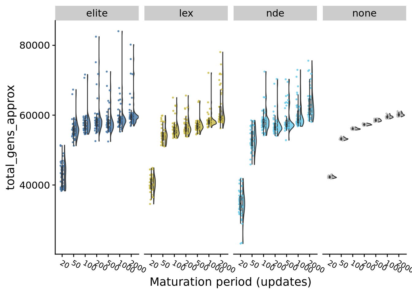
9.6 Total generations

ggplot(
    exp_summary_data,
    aes(
      x=U_PER_E,
      y=total_gens_approx,
      fill=SELECTION_METHOD
    )
  ) +
  geom_flat_violin(
    position = position_nudge(x = .2, y = 0),
    alpha = .8
  ) +
  geom_point(
    mapping=aes(color=SELECTION_METHOD),
    position = position_jitter(width = .15),
    size = .5,
    alpha = 0.8
  ) +
  geom_boxplot(
    width = .1,
    outlier.shape = NA,
    alpha = 0.5
  ) +
  scale_x_discrete(
    name="Maturation period (updates)"
  ) +
  scale_fill_manual(
    values=selection_methods_smaller_set_colors
  ) +
  scale_color_manual(
    values=selection_methods_smaller_set_colors
  ) +
  facet_wrap(
    ~SELECTION_METHOD,
    nrow=1
  ) +
  theme(
    legend.position="none",
    axis.text.x = element_text(size = 9, angle=-30, hjust=0)
  )

ggsave(
  paste0(plot_directory, "total_gens_approx.pdf"),
  width=20,
  height=10
)

median(exp_summary_data$total_gens_approx) # Used for determining how many generations to run EC for

## [1] 57167.48

for (timing in levels(exp_summary_data$U_PER_E)) {
  for (sel in c("elite", "lex", "nde", "none")) {
    print(
      paste(
        timing,
        sel,
        median(filter(exp_summary_data, U_PER_E==timing & SELECTION_METHOD==sel)$total_gens_approx)
      )
    )
  }
  print(
    paste(
      timing, "overall", median(filter(exp_summary_data, U_PER_E==timing)$total_gens_approx)
    )
  )
}

## [1] "20 elite 43147.1739335885"
## [1] "20 lex 40326.621331729"
## [1] "20 nde 34664.8985648439"
## [1] "20 none 42241.9147759426"
## [1] "20 overall 41329.1233619219"
## [1] "50 elite 55827.8934160416"
## [1] "50 lex 54050.7090498438"
## [1] "50 nde 52988.0677242188"
## [1] "50 none 53201.380141823"
## [1] "50 overall 53516.4253886458"
## [1] "100 elite 57213.4452847916"
## [1] "100 lex 55465.8904301564"
## [1] "100 nde 57919.3779984376"
## [1] "100 none 56054.7031978124"
## [1] "100 overall 56331.6952407812"
## [1] "200 elite 58024.9361635417"
## [1] "200 lex 56247.7024005208"
## [1] "200 nde 56511.7579942709"
## [1] "200 none 57294.2312760416"
## [1] "200 overall 57207.1385562501"
## [1] "500 elite 57585.15895625"
## [1] "500 lex 56747.8336604167"
## [1] "500 nde 57295.9740817708"
## [1] "500 none 58521.2714651041"
## [1] "500 overall 57697.65558125"
## [1] "1000 elite 58524.5463697916"
## [1] "1000 lex 58071.5926197917"
## [1] "1000 nde 58689.3264583334"
## [1] "1000 none 59456.0870677083"
## [1] "1000 overall 58907.1638229166"
## [1] "2000 elite 59469.05634375"
## [1] "2000 lex 59366.437359375"
## [1] "2000 nde 61755.465796875"
## [1] "2000 none 60074.0713125"
## [1] "2000 overall 60021.520203125"

9.7 Performance

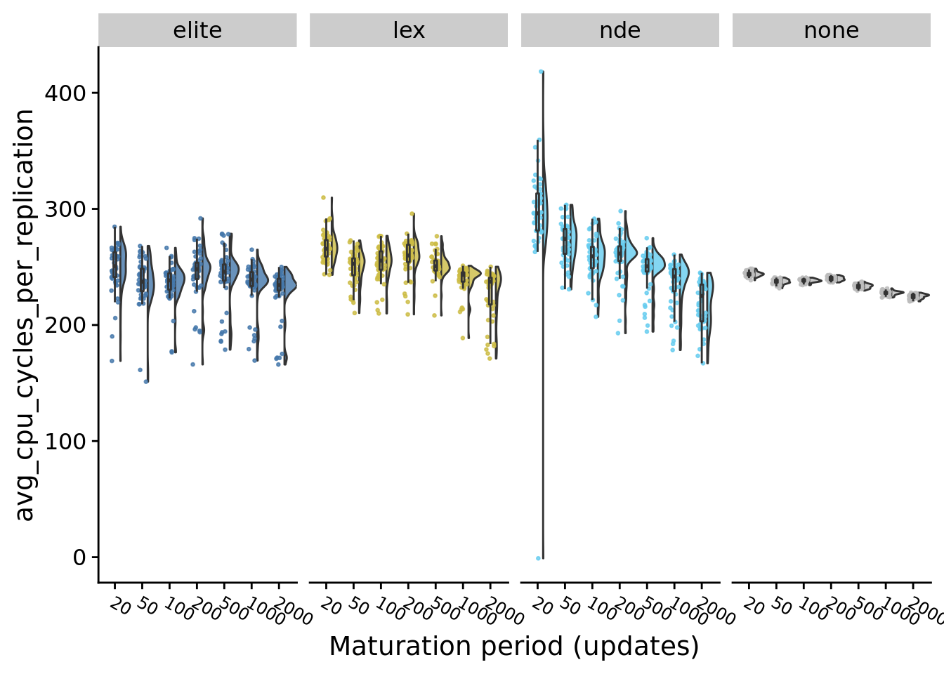
9.7.1 CPU cycles per replication

ggplot(
    exp_summary_data,
    aes(
      x=U_PER_E,
      y=avg_cpu_cycles_per_replication,
      fill=SELECTION_METHOD
    )
  ) +
  geom_flat_violin(
    position = position_nudge(x = .2, y = 0),
    alpha = .8
  ) +
  geom_point(
    mapping=aes(color=SELECTION_METHOD),
    position = position_jitter(height=0, width = .15),
    size = .5,
    alpha = 0.8
  ) +
  geom_boxplot(
    width = .1,
    outlier.shape = NA,
    alpha = 0.5
  ) +
  scale_x_discrete(
    name="Maturation period (updates)"
  ) +
  scale_fill_manual(
    values=selection_methods_smaller_set_colors
  ) +
  scale_color_manual(
    values=selection_methods_smaller_set_colors
  ) +
  facet_wrap(
    ~SELECTION_METHOD,
    scales="fixed",
    nrow=1
  ) +
  theme(
    legend.position="none",
    axis.text.x = element_text(size = 9, angle=-30, hjust=0)
  )

ggsave(
  paste0(plot_directory, "avg_cpu_cycles_per_replication.pdf"),
  width=20,
  height=10
)

9.7.2 Best-population task coverage

max_task_coverage_fig <-
  ggplot(
    exp_summary_data,
    aes(
      x=U_PER_E,
      y=max_trait_coverage,
      fill=SELECTION_METHOD
    )
  ) +
  geom_flat_violin(
    position = position_nudge(x = .2, y = 0),
    alpha = .8,
    adjust=1.5
  ) +
  geom_point(
    mapping=aes(color=SELECTION_METHOD),
    position = position_jitter(height=0.1, width = .15),
    size = .5,
    alpha = 0.8
  ) +
  geom_boxplot(
    width = .1,
    outlier.shape = NA,
    alpha = 0.5
  ) +
  scale_y_continuous(
    name="Task Coverage",
    limits=c(-0.5, 18.5),
    breaks=seq(0,18,2)
  ) +
  scale_x_discrete(
    name="Maturation period (updates)"
  ) +
  scale_fill_manual(
    values=selection_methods_smaller_set_colors
  ) +
  scale_color_manual(
    values=selection_methods_smaller_set_colors
  ) +
  facet_wrap(
    ~SELECTION_METHOD_LABEL,
    scales="fixed",
    nrow=1
  ) +
  theme(
    legend.position="none",
    axis.text.x = element_text(size = 9, angle=-30, hjust=0)
  )
max_task_coverage_fig

ggsave(
  plot=max_task_coverage_fig,
  filename=paste0(plot_directory, "max_trait_coverage.pdf"),
  width=20,
  height=10
)

for (sel in c("elite", "lex", "nde", "none")) {
  print(sel)
  sel_summary_data <- filter(exp_summary_data, SELECTION_METHOD==sel)
  kt <- kruskal.test(
    formula=max_trait_coverage~U_PER_E,
    data=sel_summary_data
  )
  print(kt)
  if (kt$p.value < 0.05) {
    pwt <- pairwise.wilcox.test(
      x=sel_summary_data$max_trait_coverage,
      g=sel_summary_data$U_PER_E,
      p.adjust.method="bonferroni",
    )
    print(pwt)
  } else {
    print("Not significant")
  }
}

## [1] "elite"
## 
##  Kruskal-Wallis rank sum test
## 
## data:  max_trait_coverage by U_PER_E
## Kruskal-Wallis chi-squared = 79.646, df = 6, p-value = 4.228e-15
## 
## 
##  Pairwise comparisons using Wilcoxon rank sum test with continuity correction 
## 
## data:  sel_summary_data$max_trait_coverage and sel_summary_data$U_PER_E 
## 
##      20      50      100     200     500     1000   
## 50   0.00055 -       -       -       -       -      
## 100  1.00000 0.05140 -       -       -       -      
## 200  0.00218 4.0e-08 0.00091 -       -       -      
## 500  0.00132 4.5e-10 0.00144 1.00000 -       -      
## 1000 0.31170 8.8e-08 0.11754 1.00000 1.00000 -      
## 2000 0.79464 2.0e-07 0.31733 0.38852 0.87304 1.00000
## 
## P value adjustment method: bonferroni 
## [1] "lex"
## 
##  Kruskal-Wallis rank sum test
## 
## data:  max_trait_coverage by U_PER_E
## Kruskal-Wallis chi-squared = 231.66, df = 6, p-value < 2.2e-16
## 
## 
##  Pairwise comparisons using Wilcoxon rank sum test with continuity correction 
## 
## data:  sel_summary_data$max_trait_coverage and sel_summary_data$U_PER_E 
## 
##      20      50      100     200     500     1000   
## 50   1.00000 -       -       -       -       -      
## 100  4.2e-11 3.8e-10 -       -       -       -      
## 200  < 2e-16 < 2e-16 1.5e-08 -       -       -      
## 500  < 2e-16 4.1e-16 4.3e-07 1.00000 -       -      
## 1000 < 2e-16 3.8e-16 5.3e-06 0.91939 1.00000 -      
## 2000 2.3e-16 1.6e-15 0.07905 2.3e-05 0.00081 0.01194
## 
## P value adjustment method: bonferroni 
## [1] "nde"
## 
##  Kruskal-Wallis rank sum test
## 
## data:  max_trait_coverage by U_PER_E
## Kruskal-Wallis chi-squared = 39.526, df = 6, p-value = 5.644e-07
## 
## 
##  Pairwise comparisons using Wilcoxon rank sum test with continuity correction 
## 
## data:  sel_summary_data$max_trait_coverage and sel_summary_data$U_PER_E 
## 
##      20      50      100     200     500     1000   
## 50   0.37356 -       -       -       -       -      
## 100  1.00000 0.00021 -       -       -       -      
## 200  1.00000 0.00023 1.00000 -       -       -      
## 500  1.00000 0.00280 1.00000 1.00000 -       -      
## 1000 1.00000 0.00471 1.00000 1.00000 1.00000 -      
## 2000 0.47187 9.1e-07 1.00000 1.00000 0.91202 0.05453
## 
## P value adjustment method: bonferroni 
## [1] "none"
## 
##  Kruskal-Wallis rank sum test
## 
## data:  max_trait_coverage by U_PER_E
## Kruskal-Wallis chi-squared = 326.54, df = 6, p-value < 2.2e-16
## 
## 
##  Pairwise comparisons using Wilcoxon rank sum test with continuity correction 
## 
## data:  sel_summary_data$max_trait_coverage and sel_summary_data$U_PER_E 
## 
##      20      50      100     200     500     1000  
## 50   0.9092  -       -       -       -       -     
## 100  < 2e-16 < 2e-16 -       -       -       -     
## 200  < 2e-16 < 2e-16 3.3e-15 -       -       -     
## 500  < 2e-16 < 2e-16 < 2e-16 1.6e-12 -       -     
## 1000 < 2e-16 < 2e-16 < 2e-16 3.7e-16 4.5e-06 -     
## 2000 < 2e-16 < 2e-16 < 2e-16 < 2e-16 1.2e-13 0.0013
## 
## P value adjustment method: bonferroni

9.7.3 Metapopulation task coverage

total_task_coverage_fig <-
  ggplot(
    exp_summary_data,
    aes(
      x=U_PER_E,
      y=total_trait_coverage,
      fill=SELECTION_METHOD
    )
  ) +
  geom_flat_violin(
    position = position_nudge(x = .2, y = 0),
    alpha = .8,
    adjust=1.5
  ) +
  geom_point(
    mapping=aes(color=SELECTION_METHOD),
    position = position_jitter(height=0.1, width = .15),
    size = .5,
    alpha = 0.8
  ) +
  geom_boxplot(
    width = .1,
    outlier.shape = NA,
    alpha = 0.5
  ) +
  scale_y_continuous(
    name="Task Coverage",
    limits=c(-0.5, 18.5),
    breaks=seq(0,18,2)
  ) +
  scale_x_discrete(
    name="Maturation period (updates)"
  ) +
  scale_fill_manual(
    values=selection_methods_smaller_set_colors
  ) +
  scale_color_manual(
    values=selection_methods_smaller_set_colors
  ) +
  facet_wrap(
    ~SELECTION_METHOD_LABEL,
    scales="fixed",
    nrow=1
  ) +
  theme(
    legend.position="none",
    axis.text.x = element_text(size = 9, angle=-30, hjust=0)
  )
total_task_coverage_fig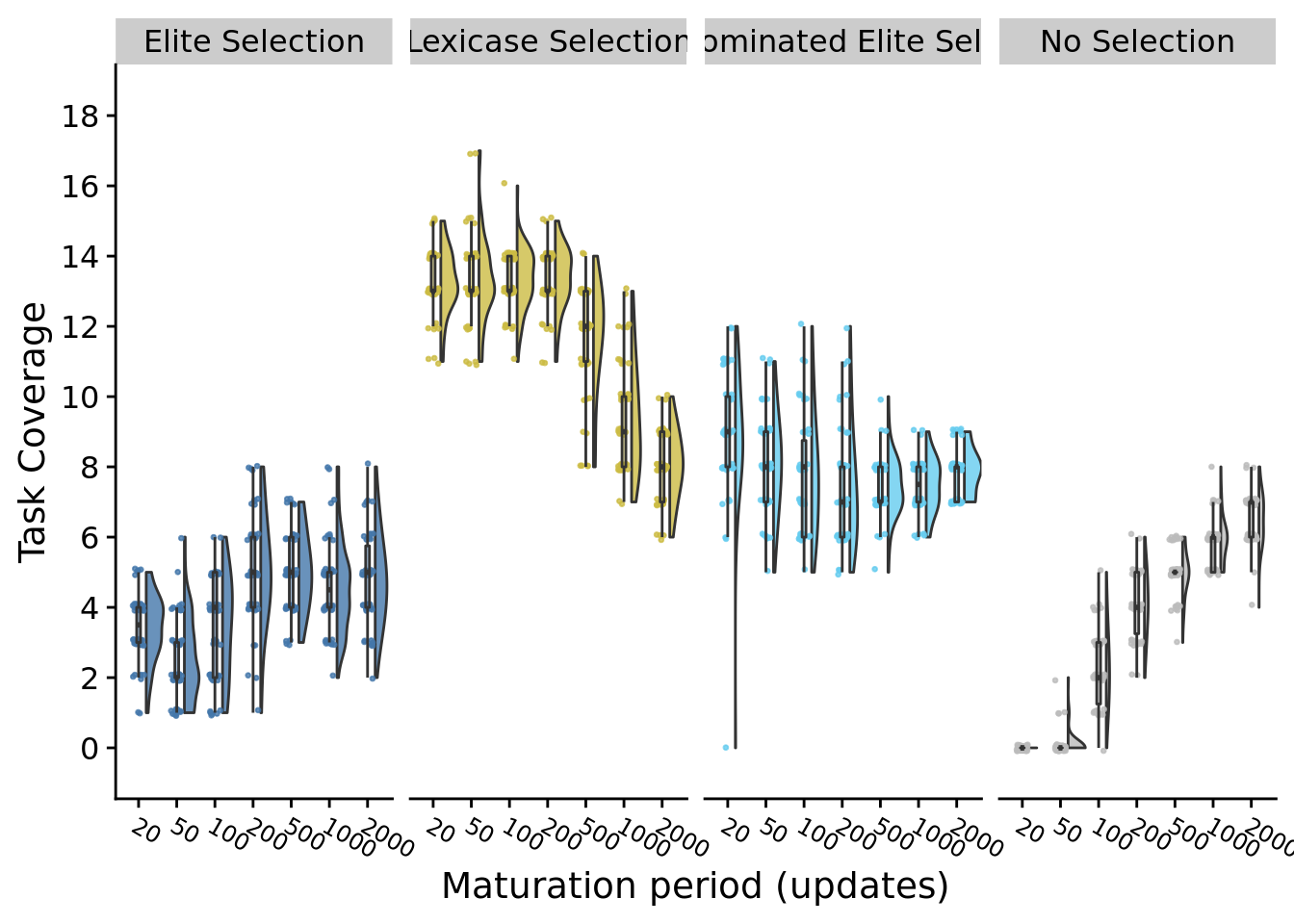

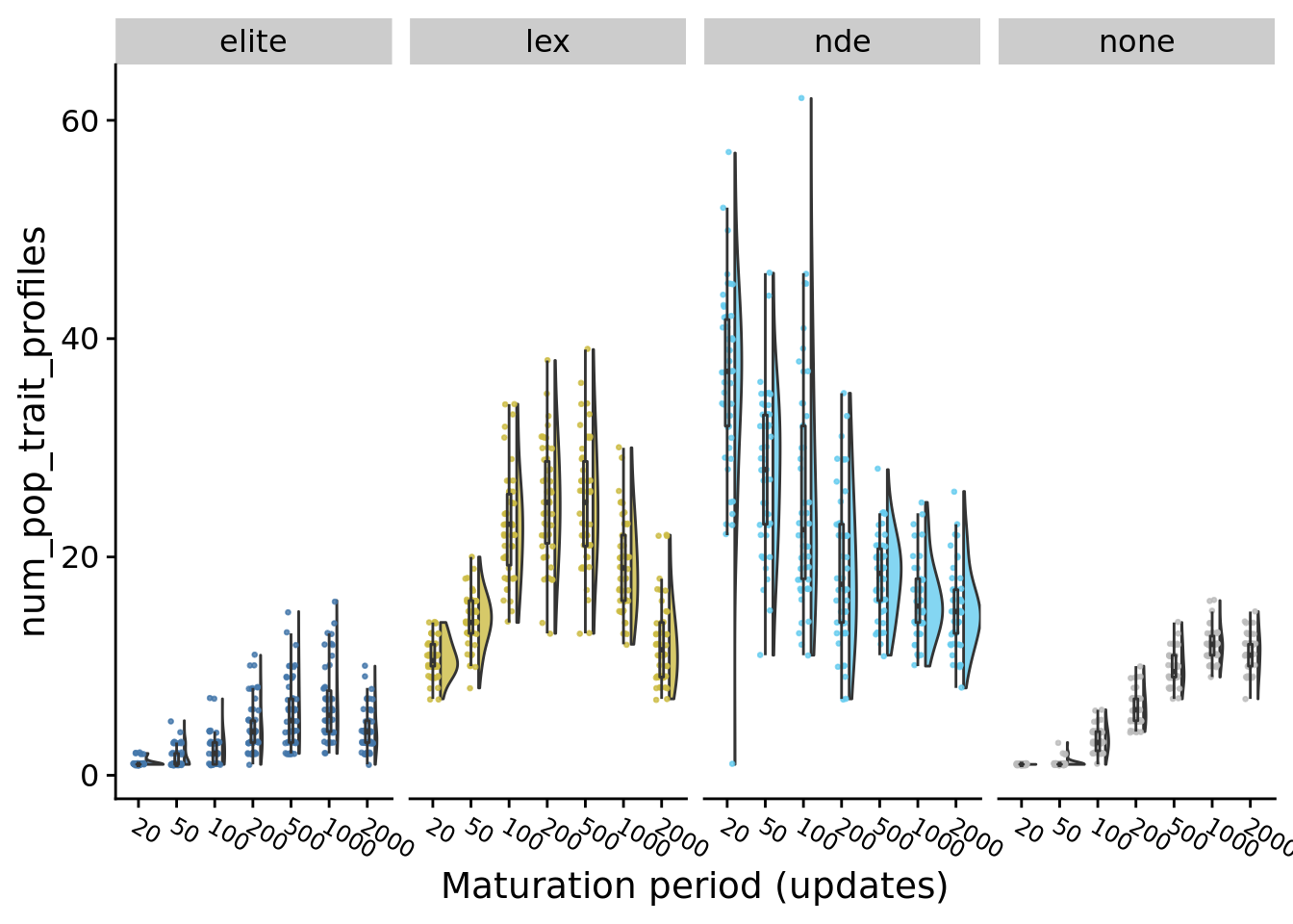
ggsave(
  plot=total_task_coverage_fig,
  filename=paste0(plot_directory, "total_trait_coverage.pdf"),
  width=20,
  height=10
)

9.8 Population-level Task Profile Diversity

9.8.1 Task profile richness

ggplot(
    exp_summary_data,
    aes(
      x=U_PER_E,
      y=num_pop_trait_profiles,
      fill=SELECTION_METHOD
    )
  ) +
  geom_flat_violin(
    position = position_nudge(x = .2, y = 0),
    alpha = .8,
    adjust=1.5
  ) +
  geom_point(
    mapping=aes(color=SELECTION_METHOD),
    position = position_jitter(height=0.1, width = .15),
    size = .5,
    alpha = 0.8
  ) +
  geom_boxplot(
    width = .1,
    outlier.shape = NA,
    alpha = 0.5
  ) +
  scale_fill_manual(
    values=selection_methods_smaller_set_colors
  ) +
  scale_color_manual(
    values=selection_methods_smaller_set_colors
  ) +
  xlab("Maturation period (updates)") +
  facet_wrap(
    ~SELECTION_METHOD,
    scales="fixed",
    nrow=1
  ) +
  theme(
    legend.position="none",
    axis.text.x = element_text(size = 9, angle=-30, hjust=0)
  )

ggsave(
  paste0(plot_directory, "num_pop_trait_profiles_facet_sel.pdf"),
  width=20,
  height=10
)

9.8.2 Task profile entropy

ggplot(
    exp_summary_data,
    aes(
      x=U_PER_E,
      y=pop_trait_profile_entropy,
      fill=SELECTION_METHOD
    )
  ) +
  geom_flat_violin(
    position = position_nudge(x = .2, y = 0),
    alpha = .8,
    adjust=1.5
  ) +
  geom_point(
    mapping=aes(color=SELECTION_METHOD),
    position = position_jitter(width = .15),
    size = .5,
    alpha = 0.8
  ) +
  geom_boxplot(
    width = .1,
    outlier.shape = NA,
    alpha = 0.5
  ) +
  scale_fill_manual(
    values=selection_methods_smaller_set_colors
  ) +
  scale_color_manual(
    values=selection_methods_smaller_set_colors
  ) +
  xlab("Maturation period (updates)") +
  facet_wrap(
    ~SELECTION_METHOD,
    scales="fixed",
    nrow=1
  ) +
  theme(
    legend.position="none",
    axis.text.x = element_text(size = 9, angle=-30, hjust=0)
  )

ggsave(
  paste0(plot_directory, "pop_trait_profile_entropy.pdf"),
  width=20,
  height=10
)

9.8.3 Spread (average cosine distance)

ggplot(
    exp_summary_data,
    aes(
      x=U_PER_E,
      y=avg_cosine_dist_from_centroid,
      fill=SELECTION_METHOD
    )
  ) +
  geom_flat_violin(
    position = position_nudge(x = .2, y = 0),
    alpha = .8,
    adjust=1.5
  ) +
  geom_point(
    mapping=aes(color=SELECTION_METHOD),
    position = position_jitter(width = .15),
    size = .5,
    alpha = 0.8
  ) +
  geom_boxplot(
    width = .1,
    outlier.shape = NA,
    alpha = 0.5
  ) +
  scale_fill_manual(
    values=selection_methods_smaller_set_colors
  ) +
  scale_color_manual(
    values=selection_methods_smaller_set_colors
  ) +
  xlab("Maturation period (updates)") +
  facet_wrap(
    ~SELECTION_METHOD,
    scales="fixed",
    nrow=1
  ) +
  theme(
    legend.position="none",
    axis.text.x = element_text(size = 9, angle=-30, hjust=0)
  )

## Warning: Removed 23 rows containing non-finite values (stat_ydensity).

## Warning: Removed 23 rows containing non-finite values (stat_boxplot).

## Warning: Removed 23 rows containing missing values (geom_point).

ggsave(
  paste0(plot_directory, "avg_cosine_dist_from_centroid_facet_sel.pdf"),
  width=20,
  height=10
)

## Warning: Removed 23 rows containing non-finite values (stat_ydensity).

## Warning: Removed 23 rows containing non-finite values (stat_boxplot).

## Warning: Removed 23 rows containing missing values (geom_point).

9.9 Selection

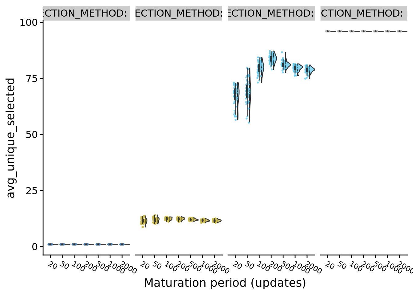
9.9.1 Average number of unique populations selected

ggplot(
    exp_summary_data,
    aes(
      x=U_PER_E,
      y=avg_unique_selected,
      fill=SELECTION_METHOD
    )
  ) +
  geom_flat_violin(
    position = position_nudge(x = .2, y = 0),
    alpha = .8
  ) +
  geom_point(
    mapping=aes(color=SELECTION_METHOD),
    position = position_jitter(height=0, width = .15),
    size = .5,
    alpha = 0.8
  ) +
  geom_boxplot(
    width = .1,
    outlier.shape = NA,
    alpha = 0.5
  ) +
  scale_x_discrete(
    name="Maturation period (updates)"
  ) +
  scale_fill_manual(
    values=selection_methods_smaller_set_colors
  ) +
  scale_color_manual(
    values=selection_methods_smaller_set_colors
  ) +
  facet_wrap(
    ~SELECTION_METHOD,
    labeller=label_both,
    nrow=1
  ) +
  theme(
    legend.position="none",
    axis.text.x = element_text(size = 9, angle=-30, hjust=0)
  )

ggsave(
  paste0(plot_directory, "avg_unique_selected_facet_sel.pdf"),
  width=20,
  height=10
)

9.9.2 Average entropy of selection ids

ggplot(
    exp_summary_data,
    aes(
      x=U_PER_E,
      y=avg_entropy_selected,
      fill=SELECTION_METHOD
    )
  ) +
  geom_flat_violin(
    position = position_nudge(x = .2, y = 0),
    alpha = .8
  ) +
  geom_point(
    mapping=aes(color=SELECTION_METHOD),
    position = position_jitter(height=0, width = .15),
    size = .5,
    alpha = 0.8
  ) +
  geom_boxplot(
    width = .1,
    outlier.shape = NA,
    alpha = 0.5
  ) +
  scale_x_discrete(
    name="Maturation period (updates)"
  ) +
  scale_fill_manual(
    values=selection_methods_smaller_set_colors
  ) +
  scale_color_manual(
    values=selection_methods_smaller_set_colors
  ) +
  facet_wrap(
    ~SELECTION_METHOD,
    scales="fixed",
    labeller=label_both
  ) +
  theme(
    legend.position="none",
    axis.text.x = element_text(size = 9, angle=-30, hjust=0)
  )

ggsave(
  paste0(plot_directory, "avg_entropy_selected.pdf")
)

## Saving 7 x 5 in image

9.10 Manuscript Figures

grid <- plot_grid(
  max_task_coverage_fig +
    theme(
      axis.text.x = element_text(size = 9, angle=-30, hjust=0),
      strip.text.x = element_text(size = 10)

    ) +
    ggtitle("Best population task coverage"),
  total_task_coverage_fig +
    theme(
      axis.text.x = element_text(size = 9, angle=-30, hjust=0),
      strip.text.x = element_text(size = 10)
    ) +
    ggtitle("Metapopulation task coverage"),
  nrow=2,
  ncol=1,
  labels="auto"
)
grid

save_plot(
  plot=grid,
  filename=paste0(plot_directory, "2021-11-12-timing-figure.pdf"),
  base_height=6
)

9.11 Discussion

Lengthening maturation period improves task coverage in the no selection control: there is more genetic variation that can build up between selection bottlenecks, which allows more population-level tasks to evolve by chance. Performance was surprisingly stable in elite and non-dominated elite selection. However, lengthening maturation period harms lexicase selection’s performance on metapopulation coverage. Overall, this experiment indicates that different selection schemes may respond differently to adjustments to the balance between individual-level and population-level selection, warranting further exploration in future work.