Chapter 27 DBSCAN in R
In this lab activity, we will do the following:
- Load and prepare data for clustering
- Apply the DBSCAN algorithm to cluster the data
- Apply the K-means algorithm to cluster the data (for comparison)
27.1 Dependencies
We’ll use the following packages in this lab activity (you will need to install any that you don’t already have installed):
library(tidyverse) # For data wrangling
library(dbscan)    # For the DBSCAN algorithm
library(cowplot)   # For ggplot theming
# Configure the default ggplot theme w/the cowplot theme.
theme_set(theme_cowplot())
27.2 Data preparation
In this lab, we’ll use some toy data in dbscan-data.csv, which you can find attached to this lab on blackboard or here.
# You will need to adjust the file path to run this locally.
data <- read_csv("lecture-material/week-10/dbscan-data.csv")
## Rows: 3695 Columns: 2
## ── Column specification ─────────────────────────────────────────────────────────────────────────────────
## Delimiter: ","
## dbl (2): x, y
##
## ℹ Use `spec()` to retrieve the full column specification for this data.
## ℹ Specify the column types or set `show_col_types = FALSE` to quiet this message.First, let’s take a look at the raw data:
ggplot(
    data,
    aes(x=x, y=y)
  ) +
  geom_point()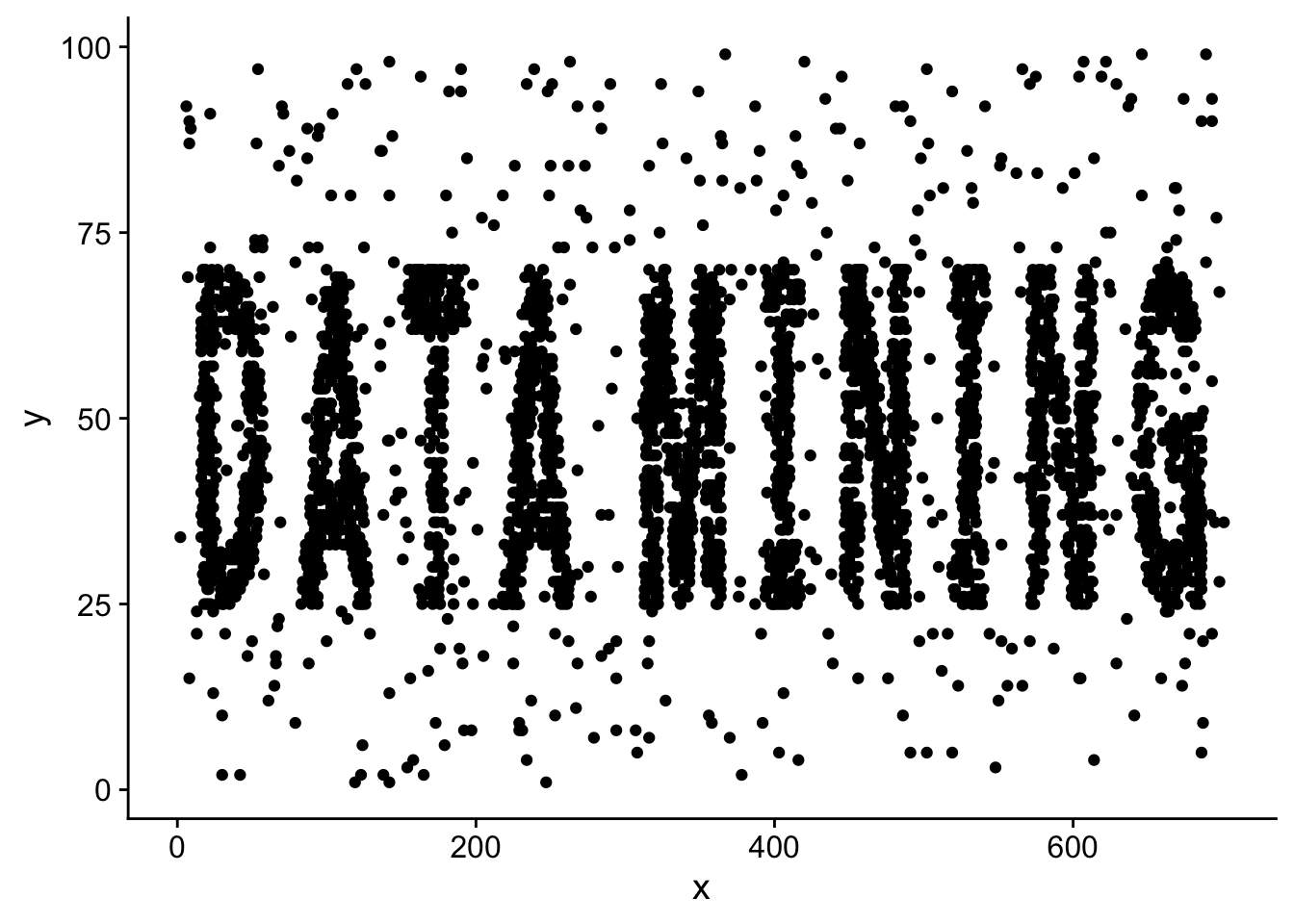
Next, let’s standardize each of the attributes we are going to use for clustering.
data$x <- scale(data$x)
data$y <- scale(data$y)
Just to see exactly what the scaling did, we can plot our data again post-standardization:
ggplot(
    data,
    aes(x=x, y=y)
  ) +
  geom_point()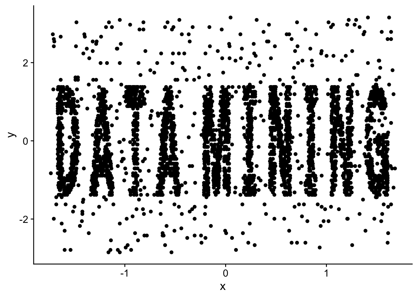
27.3 Running DBSCAN
The DBSCAN algorithm has two parameters: eps and minPts. DBSCAN assigns each data point to one of the three following categories:
- A point is a core point if it has more than a specified number of neighbors (minPts) within Eps (including itself).
- A point is a border point if it has fewer than minPts within Eps, but it is in the neighborhood of a core point.
- A point is a noise point if it is not a core point or a border point.
DBSCAN is fairly sensitive to the values you choose for the eps and minPts parameters.
For a given value of minPts, you can try to identify a good value for the eps parameter by creating a k-distance graph, which plots the distance each point is to its Kth nearest neighbor, sorted from smallest to largest.
We can use the handy kNNdistplot function (from the dbscan package) to easily create a k-nearest neighbor distance plot.
In general, a good value of eps is right around where you see an elbow in the plot.
As you increase eps, DBSCAN will generally produce fewer, bigger clusters.
eps_plot_k5 <- kNNdistplot(data, k=5)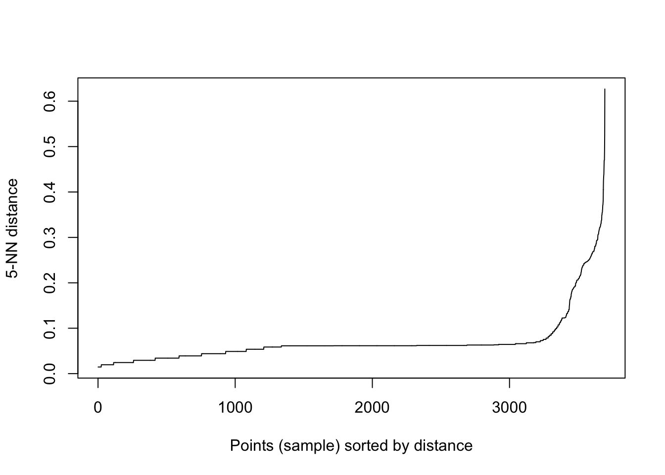
Based on the plot above, we might choose to configure our DBSCAN algorithm as follows:
# Run dbscan
results <- dbscan(
  data,
  eps = 0.075,
  minPts = 5
)
# make new dataframe with data in it so we don't add cluster id to original dataset
dbscan_data <- data
dbscan_data$cluster_id <- results$cluster
dbscan_data$cluster_id <- as.factor(dbscan_data$cluster_id)
We can plot data again, but this time we’ll color each point based on its cluster ID.
ggplot(
    dbscan_data,
    aes(x = x, y = y)
  ) +
  geom_point(
    aes(color = cluster_id)
  ) +
  ggtitle("DBSCAN Results") +
  theme(
    legend.position = "bottom"
  )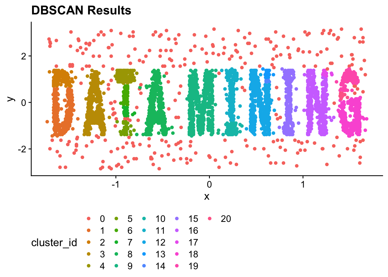
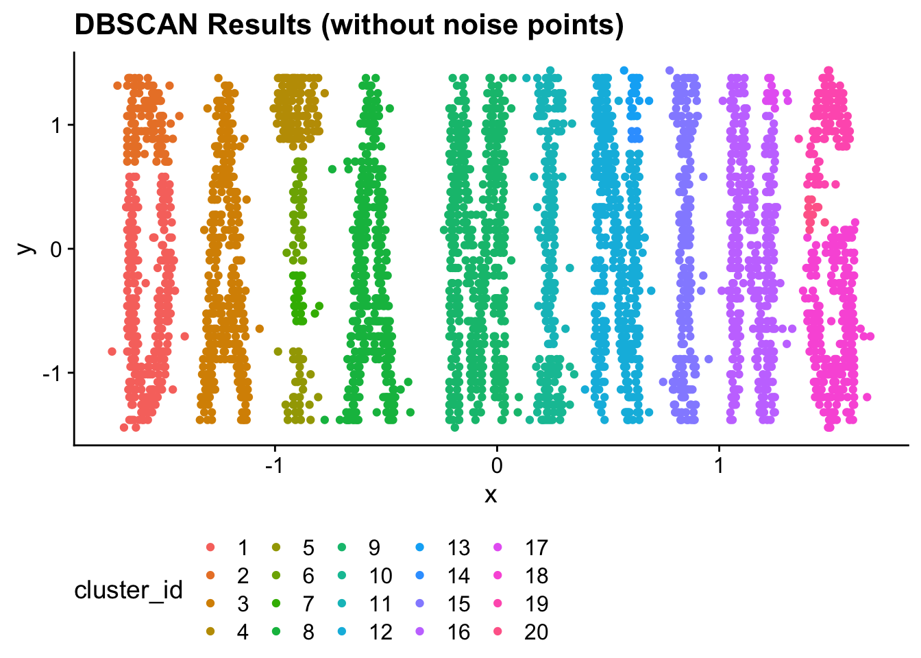
Note that all points in the “0” cluster are noise points. All other cluster IDs are real clusters. If we wanted to graph all of the clustered data points (i.e., exclude noise), we could use the dplyr filter function.
ggplot(
    filter(
      dbscan_data,
      cluster_id != 0
    ),
    aes(x = x, y = y)
  ) +
  geom_point(
    aes(color = cluster_id)
  ) +
  ggtitle("DBSCAN Results (without noise points)") +
  theme(
    legend.position = "bottom"
  )
27.4 Running K-means for comparison
Next, let’s see how K-means would have done on this data. We’ll set K equal to the number of clusters found by DBSCAN
# Calculate K from the number of cluster IDs found by DBSCAN.
# Substract 1 because cluster ID 0 represents noise points (not a cluster)
k <- length(levels(dbscan_data$cluster_id))-1
kmeans_results <- kmeans(
  data,
  centers=k
)
kmeans_data <- data
kmeans_data$cluster_id <- kmeans_results$cluster
kmeans_data$cluster_id <- as.factor(kmeans_data$cluster_id)
We’ll plot the K-means cluster results:
ggplot(
    kmeans_data,
    aes(x = x, y = y)
  ) +
  geom_point(
    aes(color = cluster_id)
  ) +
  ggtitle("K-means clustering results")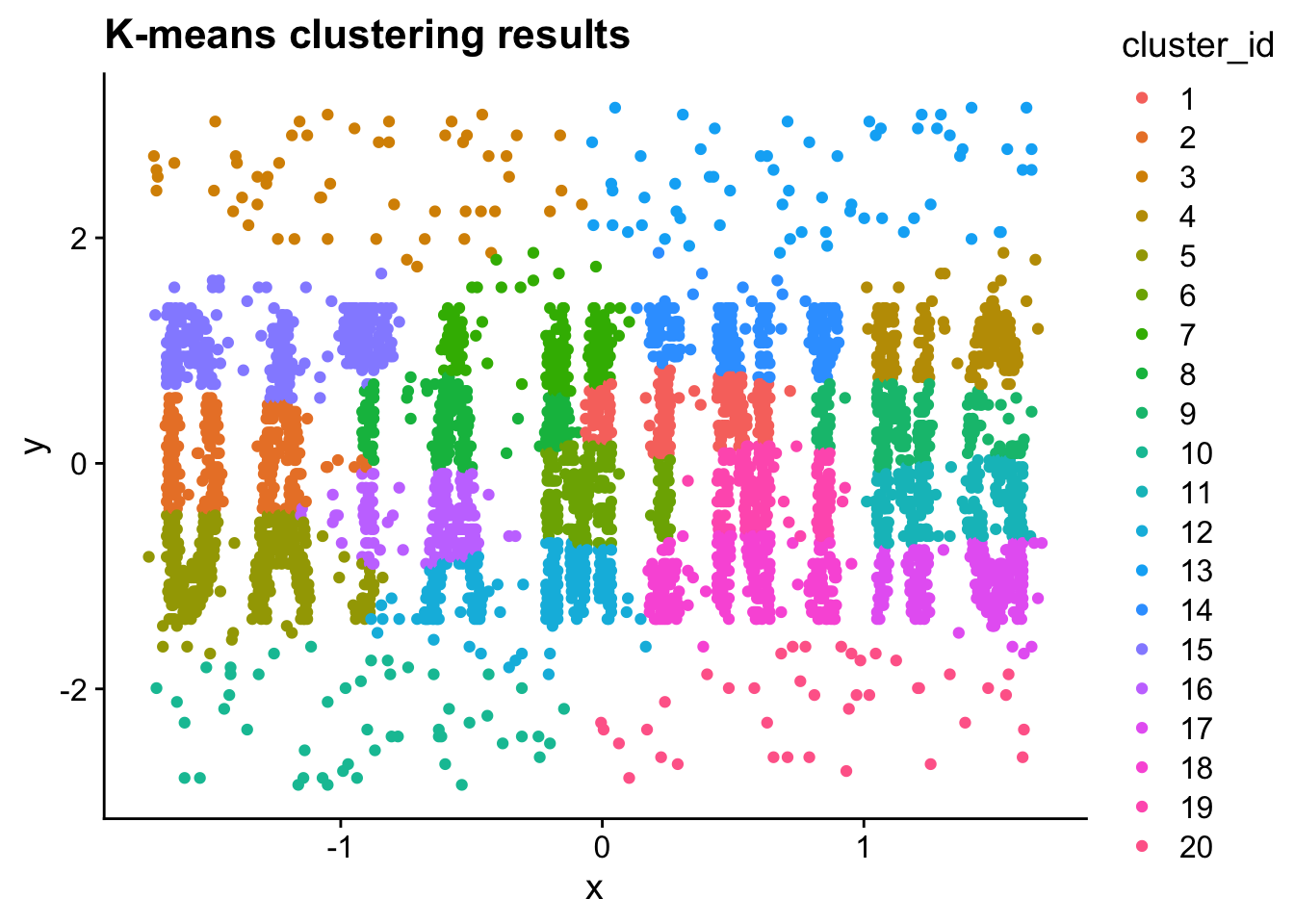
  theme(
    legend.position = "bottom"
  )
## List of 1
## $ legend.position: chr "bottom"
## - attr(*, "class")= chr [1:2] "theme" "gg"
## - attr(*, "complete")= logi FALSE
## - attr(*, "validate")= logi TRUE27.5 Exercises
- Compare the DBSCAN clustering results with the K-means clustering results. In what ways are they different? Explain why you think they are so different.
- DBSCAN is very sensitive to the values you choose for eps and minPts. What happens if you rerun DBSCAN with different values for eps and minPts? Can you configure DBSCAN to classify every point as noise? Can you configure DBSCAN to classify every point as a core point?
- Try applying a hierarchical clustering algorithm to the data in this lab (see the hierachical clustering lab activity for how to do this). How is it different/similar to the DBSCAN and the K-means results?
27.6 References
- Hahsler, M., Piekenbrock, M., & Doran, D. (2019). dbscan: Fast Density-Based Clustering with R. Journal of Statistical Software, 91(1), 1–30. https://doi.org/10.18637/jss.v091.i01