Chapter 15 Sampling objects in a dataset
In this lab activity, we will demonstrate two methods of sampling objects in a dataset:
- Naive random sampling
- Stratified random sampling
Sampling is a common method of dealing with a huge number of objects/observations in a dataset.
15.1 Dependencies and setup
In this activity, we’ll be using the following R packages:
library(tidyverse)We’ll sample from our handy-dandy Star Wars data set:
head(starwars)## # A tibble: 6 × 14
## name height mass hair_…¹ skin_…² eye_c…³ birth…⁴ sex gender homew…⁵
## <chr> <int> <dbl> <chr> <chr> <chr> <dbl> <chr> <chr> <chr>
## 1 Luke Skywal… 172 77 blond fair blue 19 male mascu… Tatooi…
## 2 C-3PO 167 75 <NA> gold yellow 112 none mascu… Tatooi…
## 3 R2-D2 96 32 <NA> white,… red 33 none mascu… Naboo
## 4 Darth Vader 202 136 none white yellow 41.9 male mascu… Tatooi…
## 5 Leia Organa 150 49 brown light brown 19 fema… femin… Aldera…
## 6 Owen Lars 178 120 brown,… light blue 52 male mascu… Tatooi…
## # … with 4 more variables: species <chr>, films <list>, vehicles <list>,
## # starships <list>, and abbreviated variable names ¹hair_color, ²skin_color,
## # ³eye_color, ⁴birth_year, ⁵homeworld15.2 Random sampling
In naive random sampling, we simply randomly sample rows from our dataset. In this example, we’ll sample without replacement: we don’t want to characters more than once in our down-sampled dataset.
sample_proportion <- 0.2 # Down-sample down to just this % of our full data set
sample_size <- ceiling(sample_proportion * nrow(starwars)) # Sample size, round up.
We can use slice_sample from the dplyr package to randomly sample star wars characters.
naive_sampled_data <- starwars %>%
  slice_sample(
    n=sample_size,
    replace=FALSE
  )
naive_sampled_data
## # A tibble: 18 × 14
## name height mass hair_…¹ skin_…² eye_c…³ birth…⁴ sex gender homew…⁵
## <chr> <int> <dbl> <chr> <chr> <chr> <dbl> <chr> <chr> <chr>
## 1 Taun We 213 NA none grey black NA fema… femin… Kamino
## 2 Biggs Dark… 183 84 black light brown 24 male mascu… Tatooi…
## 3 Wat Tambor 193 48 none green,… unknown NA male mascu… Skako
## 4 San Hill 191 NA none grey gold NA male mascu… Muunil…
## 5 Barriss Of… 166 50 black yellow blue 40 fema… femin… Mirial
## 6 Poe Dameron NA NA brown light brown NA male mascu… <NA>
## 7 Tarfful 234 136 brown brown blue NA male mascu… Kashyy…
## 8 Eeth Koth 171 NA black brown brown NA male mascu… Iridon…
## 9 Ayla Secura 178 55 none blue hazel 48 fema… femin… Ryloth
## 10 Wicket Sys… 88 20 brown brown brown 8 male mascu… Endor
## 11 Tion Medon 206 80 none grey black NA male mascu… Utapau
## 12 Arvel Cryn… NA NA brown fair brown NA male mascu… <NA>
## 13 Roos Tarpa… 224 82 none grey orange NA male mascu… Naboo
## 14 Rugor Nass 206 NA none green orange NA male mascu… Naboo
## 15 Saesee Tiin 188 NA none pale orange NA male mascu… Iktotch
## 16 Yarael Poof 264 NA none white yellow NA male mascu… Quermia
## 17 Wedge Anti… 170 77 brown fair hazel 21 male mascu… Corell…
## 18 Cliegg Lars 183 NA brown fair blue 82 male mascu… Tatooi…
## # … with 4 more variables: species <chr>, films <list>, vehicles <list>,
## # starships <list>, and abbreviated variable names ¹hair_color, ²skin_color,
## # ³eye_color, ⁴birth_year, ⁵homeworldTake a look at naive_sampled_data.
What are some ways that our random sample might not be representative of our larger data set (starwars)?
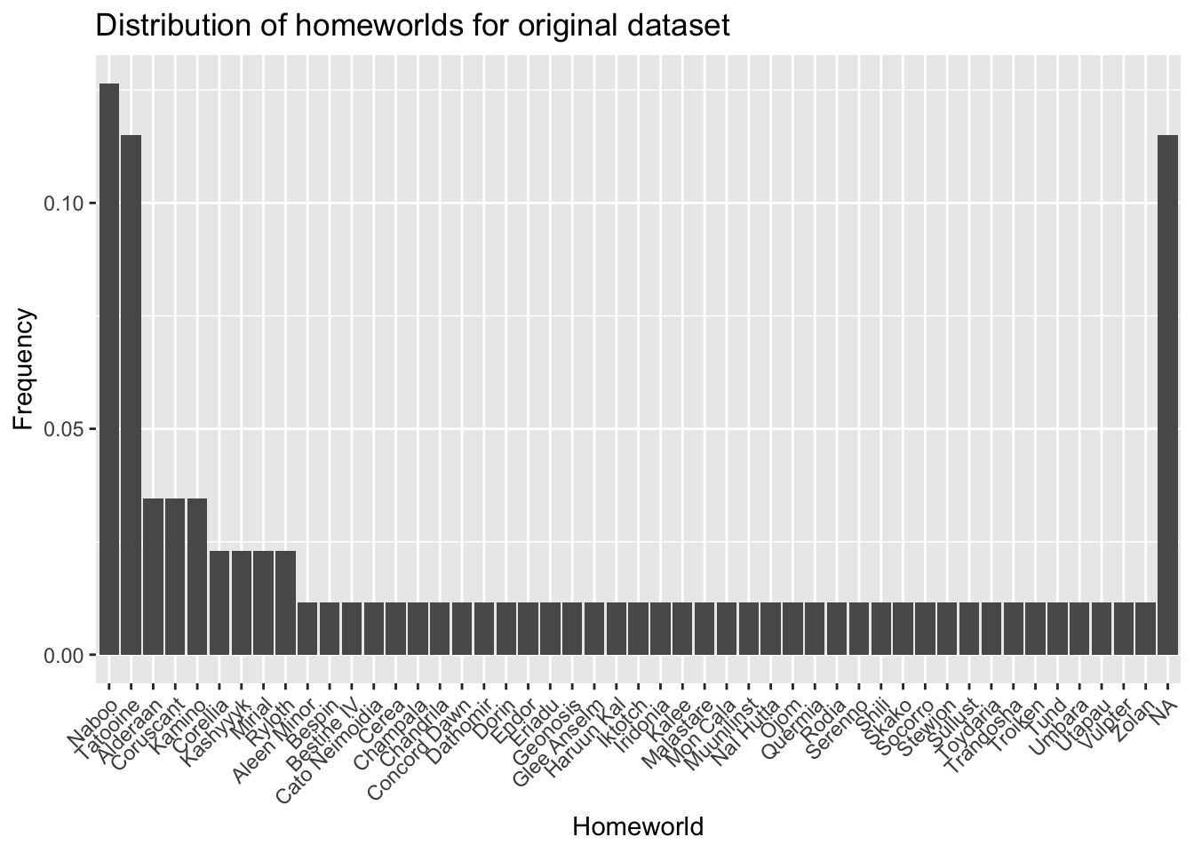
For example, we can look at the distribution of homeworlds in our original data.
# Get the distribution of homeworlds in full dataset.
orig_homeworlds <- starwars %>%
  group_by(
    homeworld
  ) %>%
  summarise(
    n=n()
  ) %>%
  mutate(
    freq = n / sum(n),
  ) %>%
  arrange(
    desc(freq)
  )

# Get the distribution of homeworlds in the sampled dataset.
sampled_homeworlds <- naive_sampled_data %>%
  group_by(
    homeworld
  ) %>%
  summarise(
    n=n()
  ) %>%
  mutate(
    freq = n / sum(n),
  ) %>%
  arrange(
    desc(freq)
  )
Let’s take a look at the distribution of homeworlds from the original dataset:
ggplot(
    orig_homeworlds,
    aes(
      x=reorder(homeworld, -freq),
      y=freq
    )
  ) +
  geom_bar(stat="identity") +
  labs(
    x="Homeworld",
    y="Frequency",
    title="Distribution of homeworlds for original dataset"
  ) +
  theme(
    axis.text.x=element_text(angle=45, hjust=1)
  )
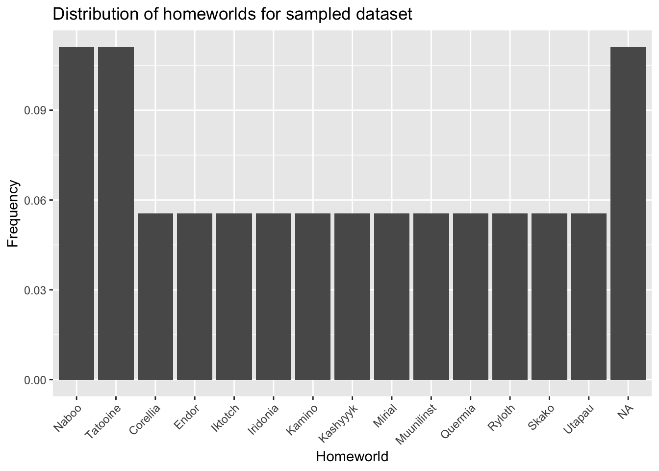
And now the sampled dataset:
ggplot(
    sampled_homeworlds,
    aes(
      x=reorder(homeworld, -freq),
      y=freq
    )
  ) +
  geom_bar(stat="identity") +
  labs(
    x="Homeworld",
    y="Frequency",
    title="Distribution of homeworlds for sampled dataset"
  ) +
  theme(
    axis.text.x=element_text(angle=45, hjust=1)
  )
15.2.1 Exercises
- What differences do you notice between the distribution of homeworlds in the original dataset and the sampled dataset?
- How could you modify
slice_sampleto randomly sample, but instead of weighting all rows equally, you weight each row’s likelihood of being included in the sample according to the height attribute? Hint:?slice_sample - Adjust the sample proportion parameter and resample. What happens to the distribution of
speciesas you increase or decrease the sample size? - Read the R code. Identify any lines of code that you don’t understand. Use the documentation to figure out what those lines of code are doing.
15.3 Stratified random sampling
Stratified sampling can be used in cases where there are predefined groupings of objects. In stratified sampling, you enforce the level of representation for each group.
For example, we might want to ensure that each species among Star Wars characters is represented in our sample. There are many ways to implement this, and the particular approach you take will depend on your objective. In this example, I’ll randomly sample each species independently, guaranteeing that at least one character of each species is represented in our sample.
# Grab the set of species represented in our original dataset
species <- levels(as.factor(starwars$species))
# Create an empty data frame that we will store our sample
stratified_sampled_data <- data.frame(
  matrix(
    ncol=ncol(starwars),
    nrow=0,
    dimnames=list(NULL,colnames(starwars))
  )
)
for (s in species) {
  # First, filter down to the species
  species_sample <- starwars %>%
    filter(
      species==s
    )
  # Calculate sample size, guarantee >= 1
  sample_size = max(
    ceiling(nrow(species_sample)*sample_proportion),
    1
  )
  # Sample from characters of the current species
  species_sample <- species_sample %>%
    slice_sample(
      n=sample_size,
      replace=FALSE
    )
  # Add sample of this species to larger sample
  stratified_sampled_data <- rbind(
    stratified_sampled_data,
    species_sample
  )
}
stratified_sampled_data
## # A tibble: 44 × 14
## name height mass hair_…¹ skin_…² eye_c…³ birth…⁴ sex gender homew…⁵
## <chr> <int> <dbl> <chr> <chr> <chr> <dbl> <chr> <chr> <chr>
## 1 Ratts Tyer… 79 15 none grey, … unknown NA male mascu… Aleen …
## 2 Dexter Jet… 198 102 none brown yellow NA male mascu… Ojom
## 3 Ki-Adi-Mun… 198 82 white pale yellow 92 male mascu… Cerea
## 4 Mas Amedda 196 NA none blue blue NA male mascu… Champa…
## 5 Zam Wesell 168 55 blonde fair, … yellow NA fema… femin… Zolan
## 6 R5-D4 97 32 <NA> white,… red NA none mascu… Tatooi…
## 7 R2-D2 96 32 <NA> white,… red 33 none mascu… Naboo
## 8 Sebulba 112 40 none grey, … orange NA male mascu… Malast…
## 9 Wicket Sys… 88 20 brown brown brown 8 male mascu… Endor
## 10 Poggle the… 183 80 none green yellow NA male mascu… Geonos…
## # … with 34 more rows, 4 more variables: species <chr>, films <list>,
## # vehicles <list>, starships <list>, and abbreviated variable names
## # ¹hair_color, ²skin_color, ³eye_color, ⁴birth_year, ⁵homeworld15.3.1 Exercises
- Graph the distribution of species in the original
starwarsdataset and in the stratified sample (just like we did for homeworlds in the naive random sample). What differences do you notice? What might be causing those differences? - We specified a sample proportion of 0.2. Why might the size of our stratified sample differ from the size of our random sample?
- Read the R code. Identify any lines of code that you don’t understand. Use the documentation to figure out what those lines of code are doing.