Chapter 2 Getting Started with R Markdown
R markdown documents are a way to interweave markdown with R. This enables us to write nicely formatted documents with R code (and output from your R code) embedded directly in the document. Find examples of compiled R markdown documents here: https://rmarkdown.rstudio.com/gallery.html In fact, this page is generated with R Markdown! Source code for this page here.
2.1 Dependencies
To use R markdown, you’ll need to install the following packages: markdown and rmarkdown. You should also want to go ahead and install the tinytex package (+ install TinyTex) to be able generate PDF output from your R Markdown documents. See the instructions below!
2.1.1 Installing R packages
As previously mentioned, there are many R packages (> 18,000!) with all sorts of useful functionality.
To install an R package, use the install.packages function in your R console (e.g., in RStudio).
Run ?install.packages in your R console to read its help page.
To install the markdown and rmarkdown packages, run the following command in your R console:
install.packages(c("markdown", "rmarkdown"))Once the installations finish, you should be able to run the following two commands without errors:
library(markdown)
library(rmarkdown)
For this class, you’ll also need to be able to generate PDF output from your R Markdown documents. To do so, you’ll need to instal LaTex (if you’re not sure what that is, no worries!). Run the following two commands in your R console in RStudio:
install.packages('tinytex')
tinytex::install_tinytex()
2.2 Create a new R Markdown document in RStudio
Click the new file button in the top right of the RStudio window, and select R Markdown.
In RStudio, you should get a pop-up for creating a new r markdown document. For now, there are two relevant options:
- Click the “Create Empty Document” in the bottom left of the popup. This will create an empty R markdown file for you.
- Fill out the title, author (you!), and date fields and press “Okay”. This will create a new R markdown file, but RStudio will initialize your file with a bunch of stuff (this stuff is helpful information, but you will want to delete it all for any assignments in this class).
2.3 Anatomy of an R Markdown document
There are three basic components in an R Markdown document: the metadata, text, and code.
Here’s the contents for a minimal R Markdown document (from https://bookdown.org/yihui/rmarkdown/basics.html):
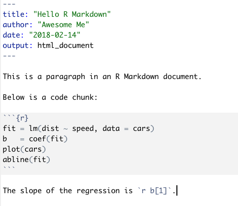
An R Markdown document should be a plain text file (i.e., don’t try to write one in google docs or microsoft word!) and conventionally has the .Rmd file extension.
2.3.1 Frontmatter (metadata)
The metadata (or the frontmatter) specifies how your R Markdown should be compiled. E.g., the output file type, whether to include a table of contents, etc.
The metadata should be written between a pair of three dashes --- at the top of your document (see minimal example).
For now, don’t worry too much about what you should include in your document metadata. For the most part, you can just use what RStudio includes in your document.
2.3.2 Text
The body of your document follows the metadata. Any text (i.e., everything that isn’t code) you include in your document should follow markdown syntax.
If you’re not already familiar with markdown, read over this: https://www.markdownguide.org/getting-started.
- For basic markdown syntax, see: https://www.markdownguide.org/basic-syntax/. Being familiar with basic syntax should be just about everything you need for your homework assignments in this class.
- For more advanced markdown syntax, see: https://www.markdownguide.org/extended-syntax/.
- You can also refer to Section 2.5 in R Markdown: The Definitive Guide for more info on markdown.
2.3.3 Code
In general, you can include code in your R Markdown documents in two ways:
- Inline code begin with
`rand end with a`. E.g.,2would render the result oflog(4, base=2)inline. - You can include a “code chunk” inside your R Markdown document. A code chunk begins with three backticks
```{r}and end with three backticks (see minimal example above for an example). There are many options tha tyou can specify in the{}at the beginning of a code chunk. See https://yihui.org/knitr/options/ for details.
2.4 “Knitting”
To compile an R Markdown document into a PDF or HTML file, you need to “Knit” it. In RStudio, this is pretty straightforward. Just click the “Knit” button on your document in RStudio.
2.5 Resources
- R Markdown: The Definitive Guide
- Code chunk options: https://yihui.org/knitr/options/