Chapter 25 Simple K-means clustering in R
In this lab activity, we will
- load a dataset and apply k-means clustering using the built-in
kmeansfunction in R. - use within-cluster sum of square error to help us choose a good number of clusters for the k-means algorithms
25.1 Dependencies and setup
We’ll use the following packages in this lab activity (you will need to install any that you don’t already have installed):
library(tidyverse)
library(cowplot)    # Used for ggplot plot theme
library(khroma)     # Used for color scheme for ggplot
theme_set(theme_cowplot()) # Set ggplot theme to the cowplot theme
25.2 Loading and preprocessing the data
In this lab activity, we’ll be using some toy data in points.csv, which you can find attached to this lab on blackboard or here.
# Load data from file into a tibble (a fancy data frame).
# You will need to adjust the file path to run this locally.
data <- read_csv("lecture-material/week-09/points.csv")
## Rows: 400 Columns: 2
## ── Column specification ─────────────────────────────────────────────────────────────────────────────────
## Delimiter: ","
## dbl (2): attr0, attr1
##
## ℹ Use `spec()` to retrieve the full column specification for this data.
## ℹ Specify the column types or set `show_col_types = FALSE` to quiet this message.This dataset has 400 with two numeric attributes: attr0 and attr1.
colnames(data)## [1] "attr0" "attr1"We can graph the raw data:
ggplot(
    data,
    aes(x=attr0, y=attr1)
  ) +
  geom_point()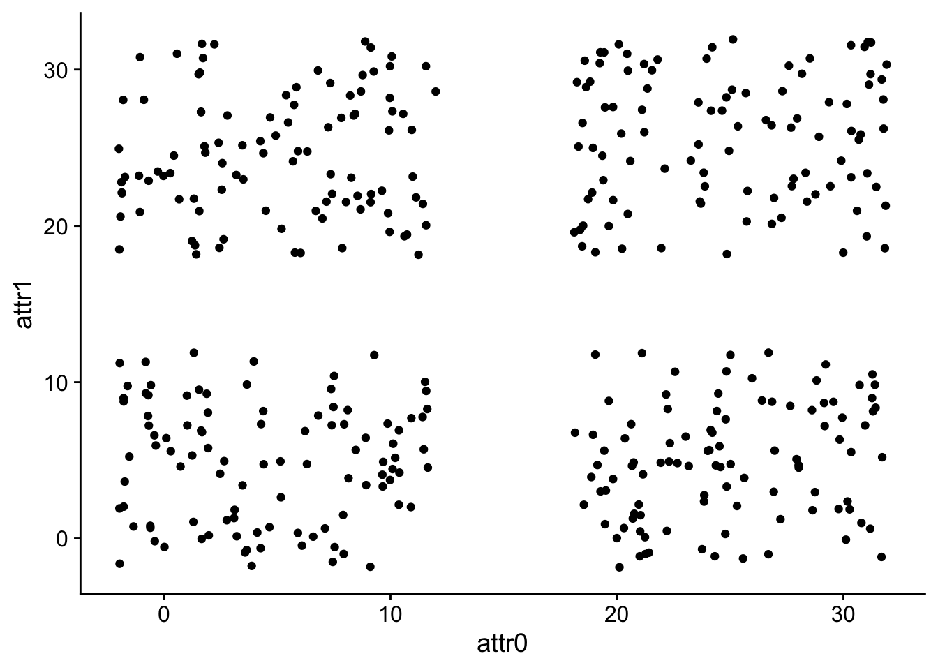
To perform k-means clustering in R, the data should almost always be prepared as follows:
- Rows are observations/objects that you want to cluster, columns are attributes
- Missing values should be removed or estimated
- Each column (attribute) should be standardized to make attributes comparable. E.g., you might standardize an attribute by tranforming the variables such that they have a mean of 0 and a standard deviation of 1.
Fortunately, our data already satisfy the first two requirements.
We just need to standardize each column, which we can do with the scale function in R:
# Run ?scale to read about how the scale function works in R
data$attr0 <- scale(data$attr0)
data$attr1 <- scale(data$attr1)
Let’s graph our data again now that we’ve scaled each column.
ggplot(
    data,
    aes(x=attr0, y=attr1)
  ) +
  geom_point()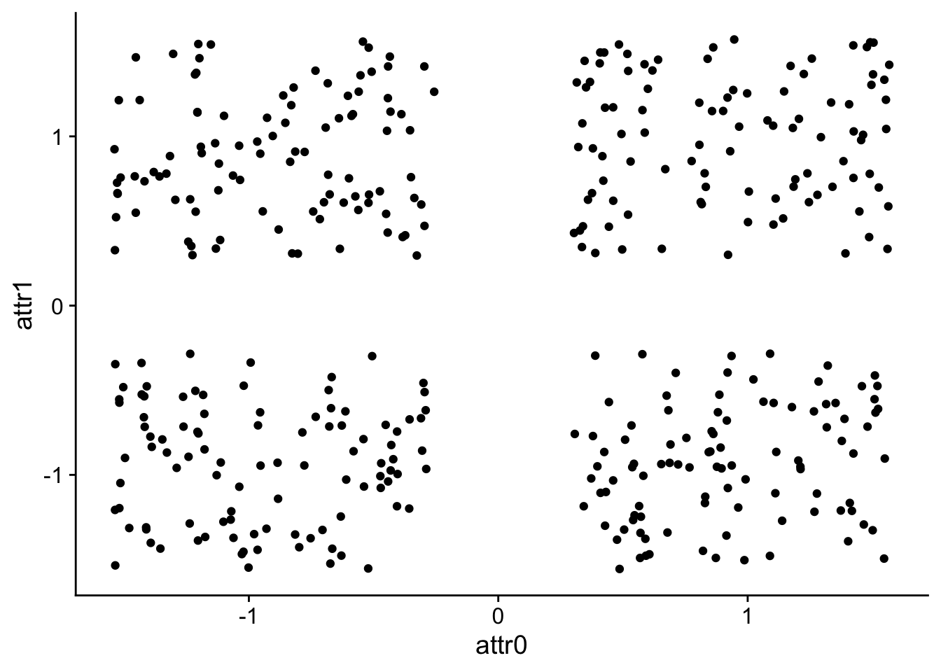
25.3 Running k-means
We can use the built-in kmeans function to perform k-means clustering in R.
kmeans only works with numeric columns.
If you want to use cluster data based on categorical/non-numeric columns, you’ll need to either convert those columns to numbers such that distances between the numeric values you convert to correspond with the distances between categories/symbols. Otherwise, you might need to look for other implementations of k-means that allows for more customization, or you might need to implement k-means yourself with your own custom distance measure.
Note that kmeans does not let you configure the distance function it uses to perform clustering.
Read more about common distance functions here: https://uc-r.github.io/kmeans_clustering#distance
Unfortunately, if you want to customize the distance function, you’ll need to find a more customizable implementation of k-means clustering or implement it yourself.
Fortunately, the k-means algorithm is fairly straightforward, making it not too bad to write your own implementation: https://uc-r.github.io/kmeans_clustering#kmeans
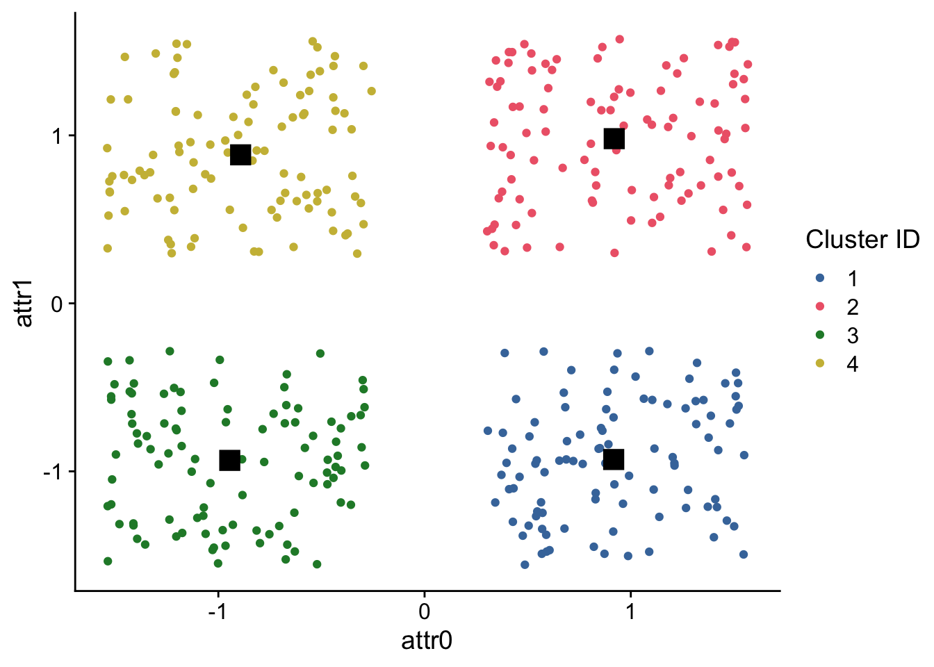
We know from looking at our raw data that it probably makes sense to cluster our data into 4 clusters:
# Run ?kmeans to read about each of the function arguments used below
cluster_results <- kmeans(
  data,
  centers = 4,              # K, number of clusters to partition data into
  iter.max = 100,
  nstart = 10,              # Try 10 different starting centroids, pick best one
  algorithm = "Lloyd"       # Particular version of kmeans algorithm
)
cluster_results
## K-means clustering with 4 clusters of sizes 100, 100, 100, 100
##
## Cluster means:
## attr0 attr1
## 1 0.9169208 -0.9296131
## 2 0.9196341 0.9803683
## 3 -0.9446068 -0.9348886
## 4 -0.8919481 0.8841333
##
## Clustering vector:
## [1] 1 2 1 1 1 1 3 3 3 1 3 3 3 3 3 4 2 3 3 3 1 3 3 2 2 2 2 4 3 3 4 3 4 1 1 1 2
## [38] 4 2 2 4 3 1 1 3 1 1 1 4 4 4 1 1 2 4 1 3 2 1 2 2 3 3 1 4 1 3 4 4 2 2 1 3 2
## [75] 1 1 4 1 1 2 2 2 1 2 3 1 4 3 2 4 1 4 1 3 1 1 2 4 3 2 1 4 3 4 1 4 2 2 3 3 1
## [112] 4 4 1 4 4 1 4 2 2 4 3 1 1 4 1 2 1 4 1 2 3 3 4 4 3 1 1 4 2 4 3 2 4 2 3 2 2
## [149] 4 4 4 1 2 3 2 4 3 3 4 2 3 3 4 2 3 4 2 1 3 3 3 3 2 1 2 4 3 3 1 3 2 1 4 4 2
## [186] 2 4 2 1 2 4 4 3 2 3 3 2 3 4 4 2 2 4 3 2 4 2 4 4 3 4 4 4 2 4 3 4 1 1 1 2 2
## [223] 3 4 3 2 2 3 3 4 2 2 2 1 1 4 3 2 3 4 3 1 4 3 4 2 2 1 1 1 4 4 2 1 3 4 3 4 4
## [260] 3 1 4 2 3 2 2 1 4 1 1 4 1 1 1 3 4 1 1 4 2 1 2 4 4 4 4 2 3 2 4 1 3 4 1 2 3
## [297] 4 3 1 4 4 3 1 2 4 4 1 4 1 2 3 3 2 2 1 2 3 1 1 2 3 3 4 3 1 3 2 4 3 2 3 3 2
## [334] 1 3 3 3 4 2 1 3 2 4 4 2 1 4 1 1 1 2 4 3 4 2 2 4 3 2 1 1 1 2 3 2 2 4 1 2 2
## [371] 1 1 1 2 2 3 3 1 1 3 2 1 2 1 2 3 3 3 4 3 1 1 3 4 3 4 4 1 2 2
##
## Within cluster sum of squares by cluster:
## [1] 25.06436 32.05632 27.63571 27.71012
## (between_SS / total_SS = 85.9 %)
##
## Available components:
##
## [1] "cluster" "centers" "totss" "withinss" "tot.withinss"
## [6] "betweenss" "size" "iter" "ifault"cluster_results$cluster has the cluster ids for each row in our dataset.
To make graphing our clustered data easier, let’s add a cluster_id column to our dataset.
# Add column to data that specifies the cluster that each row belongs to
data$cluster_id <- as.factor(cluster_results$cluster)
head(data)
## # A tibble: 6 × 3
## attr0[,1] attr1[,1] cluster_id
## <dbl> <dbl> <fct>
## 1 0.821 -1.45 1
## 2 0.337 1.08 2
## 3 1.27 -0.625 1
## 4 1.42 -1.21 1
## 5 0.935 -0.297 1
## 6 0.486 -1.56 1Next, let’s graph our data but we’ll color points based on their cluster membership.
Additionally, we’ll overlay the centroids (stored in cluster_results$centers) as black squares on our data.
# Create a dataframe with cluster centers that we can plot
cluster_centers <- as.data.frame(cluster_results$centers)
head(cluster_centers)
## attr0 attr1
## 1 0.9169208 -0.9296131
## 2 0.9196341 0.9803683
## 3 -0.9446068 -0.9348886
## 4 -0.8919481 0.8841333ggplot(
data,
aes(
x = attr0,
y = attr1,
color = cluster_id,
fill = cluster_id
)
) +
geom_point() +
geom_point(
data=cluster_centers,
shape=15,
fill="black",
color="black",
size=5
) +
scale_color_bright(
name = "Cluster ID"
) +
scale_fill_bright(
name = "Cluster ID"
)
You are not guaranteed to get the same clusters everytime you run k-means. The clusters you end up can change depending on the initial centroids chosen.
25.4 What if you don’t know the best number of clusters a priori?
The k-means algorithm requires that you set the number of clusters you want to partition your data into as a parameter. In the example above, we looked at the data (which was conveniently 2-dimensional), and we decided that we should have 4 clusters. But often, your data are many-dimensional, and it is obvious how many clusters you use a priori.
In these situations, we can run k-means with different values for k and choose the k that gives us the “best clustering”. But how do we assess the quality of a clustering?
There are three common methods for choosing the best number of clusters (i.e., the best value for k):
- Elbow method
- Silhouette method
- Gap statistic
Read more about each of those methods here: https://uc-r.github.io/kmeans_clustering#optimal.
Here, we’ll demonstrate the simplist of those three: the Elbow method. For the elbow method, we assess our clustering results for a particular k by measuring the within-cluster variation (i.e., total within-cluster sum of square error). The total within-cluster sum of square error measures the “compactness” of a cluster.
In the extreme, you can minimize total within-cluster sum of square error (i.e., maximize compactness) by having each individual data point in its own cluster, which results in 0 within-cluster variation. However, that’s not particularly useful from a data mining perspective. In general, you want the smallest value of k (i.e., the fewest number of clusters) where each cluster is still reasonably “compact”. If that all sounds a little vague to you, it is! With the elbow method, you plot the total within-cluster sum of square error for different values of k, and choose the k where the curve “bends” and you start getting diminishing returns in compactness for increasing k.
# wss will hold the within-cluster square error for running kmeans on our data
# for k values ranging from 2 to 10. That is, we run kmeans 9 times, once per k.
wss <- data.frame(k=integer(),wss=double())
# k_range gives the range of k values we're going to try
k_range <- 2:10
# For each k value we want to try, run kmeans and record the within-cluster square
# error.
for (k in k_range) {
  error <- kmeans(data, k, nstart=10)$tot.withinss
  wss <- rbind(wss, list("k"=k, "wss"=error))
}
head(wss)
## k wss
## 1 2 560.44901
## 2 3 328.04719
## 3 4 112.46651
## 4 5 98.45581
## 5 6 87.37497
## 6 7 75.24178Next, we plot the within-cluster squared error that we measured for each value of k that we tried.
ggplot(
    data = wss,
    mapping = aes(x=k,y=wss)
  ) +
  geom_point() +
  geom_line() +
  scale_y_continuous(
    name="Within-cluster sum of square error (wss)"
  ) +
  scale_x_continuous(
    name="k (number of clusters)",
    breaks=k_range
  )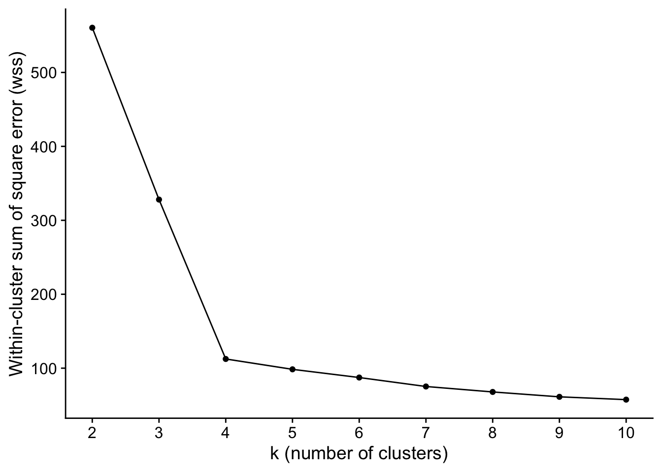
In this case, the “elbow” of the curve is pretty obvious at 4. In real-world data, it might be similarly obvious. Or, it’ll be a little less obvious, and you might run your entire data mining pipeline for a couple of decent values of k.
I strongly encourage you to read up on the other methods of choosing a good k: https://uc-r.github.io/kmeans_clustering#optimal.
25.5 Exercises
- Identify any lines of code that you do not understand. Use the documentation to figure out what is going on.
- Plot cluster assignment for running kmeans with k=2 and k=8. Compare those assignments with k=4. Which had the highest within-cluster square error? Which had the lowest? Discuss your findings.
- Discuss what you would need to do to apply k-means clustering to non-numeric data. Describe a step-by-step process by which you could use k-means clustering to cluster Tweets.
25.7 References
- https://uc-r.github.io/kmeans_clustering – If you want to go a step deeper into using k-means clustering, I strongly encourage you to work through this article (which includes R code)